1. Ce que "chaos" veut dire pour un marchéWhat "chaos" means for a market
Un marché chaotique n'est pas un marché bruyant. C'est un marché déterministe, sensible aux conditions initiales, avec un exposant de Lyapunov positif sur l'attracteur des prix renormalisés. Sur BTC/USD entre 2020 et 2025, on mesure $\lambda_1 \approx 0.05 \pm 0.01$ jour⁻¹ — soit une horizon de prédictibilité d'environ 20 jours, après lequel deux trajectoires initialement séparées de 0.1 % divergent au-delà de 100 %.
A chaotic market is not a noisy market. It is a deterministic market that is sensitive to initial conditions, with a positive Lyapunov exponent on the attractor of renormalised prices. On BTC/USD between 2020 and 2025, one measures $\lambda_1 \approx 0.05 \pm 0.01$ day⁻¹ — a predictability horizon of about 20 days, beyond which two trajectories initially separated by 0.1 % diverge past 100 %.
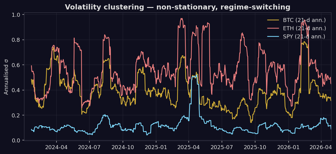
La signature observable est la volatilité par grappes : périodes calmes interrompues par des bouffées intenses, avec une distribution de durées en loi de puissance. C'est le marqueur d'un système hors équilibre proche d'une transition de phase, exactement comme la magnétisation près du point critique d'un Ising 2D.
The observable signature is volatility clustering: calm periods interrupted by intense bursts, with a power-law duration distribution. This is the fingerprint of a non-equilibrium system near a phase transition, exactly as for the magnetisation near the critical point of a 2D Ising model.
Le problème : ces modèles décrivent statistiquement le chaos sans donner de prise pour le contrôler. Pour cela il faut un cadre dynamique où l'on peut écrire une équation d'évolution du gérant de portefeuille et de son environnement. C'est exactement ce que font les jeux à champ moyen.
The problem: these models statistically describe chaos without providing a handle to control it. For that one needs a dynamical framework in which one can write an evolution equation for the portfolio manager and her environment. That is exactly what mean-field games provide.
2. McKean-Vlasov — des agents qui regardent la fouleMcKean-Vlasov — agents that watch the crowd
Un agent typique sur un actif risqué $X_t$ contrôle sa position $\alpha_t$ pour optimiser un critère $J(\alpha; \mu)$ où $\mu_t$ est la distribution empirique des positions de tous les autres. Sa dynamique est une EDS de McKean-Vlasov :
A typical agent on a risky asset $X_t$ controls her position $\alpha_t$ to optimise a criterion $J(\alpha; \mu)$ where $\mu_t$ is the empirical distribution of all other positions. Her dynamics is a McKean-Vlasov SDE:
$$dX_t \;=\; b\bigl(t, X_t, \mu_t, \alpha_t\bigr)\,dt \;+\; \sigma\bigl(t, X_t, \mu_t\bigr)\,dW_t, \qquad \mu_t \;=\; \mathcal{L}(X_t).$$
L'équilibre de Nash en jeu à champ moyen (Lasry-Lions 2007, Carmona-Delarue 2018) revient au système couplé d'une Hamilton-Jacobi-Bellman rétrograde pour la fonction valeur et d'une Fokker-Planck avant pour $\mu_t$. C'est la première marche pour modéliser une réflexivité de marché : chaque trader réagit à ce que font les autres, ce qui modifie la distribution, ce qui modifie les réactions futures. Le chaos vient de l'instabilité de ce point fixe.
The mean-field Nash equilibrium (Lasry-Lions 2007, Carmona-Delarue 2018) reduces to a coupled system of a backward Hamilton-Jacobi-Bellman for the value function and a forward Fokker-Planck for $\mu_t$. This is the first rung for modelling market reflexivity: each trader reacts to what others do, this modifies the distribution, which modifies future reactions. Chaos emerges from the instability of this fixed point.
2.1 Dérivation du système HJB–Fokker-Planck2.1 Deriving the HJB–Fokker-Planck system
L'agent représentatif minimise une fonctionnelle de coût $J(\alpha;\mu) = \mathbb{E}\!\left[\int_0^T f(X_s,\alpha_s,\mu_s)\,ds + g(X_T,\mu_T)\right]$. La fonction valeur est définie par $v(t,x) = \inf_\alpha \mathbb{E}[\cdot\mid X_t=x]$. L'application du principe de programmation dynamique de Bellman donne, en formel, $v(t,x) = \inf_\alpha \mathbb{E}[f\,dt + v(t+dt, X_{t+dt})]$. En développant par Itô :
The representative agent minimises the cost functional $J(\alpha;\mu) = \mathbb{E}\!\left[\int_0^T f(X_s,\alpha_s,\mu_s)\,ds + g(X_T,\mu_T)\right]$. The value function is $v(t,x) = \inf_\alpha \mathbb{E}[\cdot\mid X_t=x]$. Bellman's dynamic-programming principle yields, formally, $v(t,x) = \inf_\alpha \mathbb{E}[f\,dt + v(t+dt, X_{t+dt})]$. Expanding by Itô:
$$0 \;=\; \partial_t v \;+\; \inf_{\alpha}\Bigl\{\, b(t,x,\mu_t,\alpha)\cdot\nabla_x v \;+\; \tfrac{1}{2}\,\mathrm{tr}\bigl(\sigma\sigma^\top\,\nabla^2_x v\bigr) \;+\; f(x,\alpha,\mu_t) \,\Bigr\}, \qquad v(T,x)=g(x,\mu_T).$$
L'infimum atteint en $\alpha^\star(t,x,\mu_t,\nabla_x v)$ fournit le contrôle optimal en feedback. On le réinjecte dans la dynamique pour obtenir l'EDP avant pour la densité $\mu_t(x)$ (Fokker-Planck) :
The infimum, achieved at $\alpha^\star(t,x,\mu_t,\nabla_x v)$, supplies the optimal feedback control. Substituting it into the dynamics yields the forward Fokker-Planck PDE for $\mu_t(x)$:
$$\partial_t \mu_t \;+\; \nabla_x\!\cdot\!\bigl(b(t,x,\mu_t,\alpha^\star)\,\mu_t\bigr) \;-\; \tfrac{1}{2}\,\mathrm{tr}\bigl(\nabla^2_x(\sigma\sigma^\top \mu_t)\bigr) \;=\; 0, \qquad \mu_0 \text{ given.}$$
Le couple HJB rétrograde + FP avant forme le système MFG de Lasry-Lions. Le théorème principal (existence, unicité sous monotonie de Lasry-Lions) garantit qu'un équilibre de Nash en champ moyen existe et coïncide avec ce point fixe. C'est sur ce système qu'on injecte ensuite réduction dimensionnelle et invariants topologiques.
The backward HJB + forward FP couple forms the Lasry-Lions MFG system. The main theorem (existence and uniqueness under the Lasry-Lions monotonicity condition) guarantees a mean-field Nash equilibrium exists and coincides with this fixed point. Dimensional reduction and topological invariants are then layered on top of this system.
2.2 Cas linéaire-quadratique fermé2.2 Closed-form linear-quadratic case
Si la dynamique est linéaire $dX_t = (aX_t + \bar X_t b + \alpha_t)\,dt + \sigma\,dW_t$ avec $\bar X_t = \mathbb{E}[X_t]$ (interaction de champ moyen au premier moment) et le coût quadratique $f = \tfrac12 q\,x^2 + \tfrac12 r\,\alpha^2$, l'équation HJB devient une équation de Riccati pour $P(t)$ :
If dynamics are linear $dX_t = (aX_t + \bar X_t b + \alpha_t)\,dt + \sigma\,dW_t$ with $\bar X_t = \mathbb{E}[X_t]$ (first-moment mean-field interaction) and cost quadratic $f = \tfrac12 q\,x^2 + \tfrac12 r\,\alpha^2$, the HJB collapses to a Riccati equation for $P(t)$:
$$\dot P(t) \;+\; 2a\,P(t) \;-\; \tfrac{1}{r}\,P(t)^2 \;+\; q \;=\; 0, \qquad P(T)=q_T,$$
avec la solution explicite (en supposant $a^2 + q/r > 0$, $\Delta = \sqrt{a^2 r + q\,r}$) :
with explicit solution (assuming $a^2 + q/r > 0$, $\Delta = \sqrt{a^2 r + q\,r}$):
$$P(t) \;=\; \Delta \cdot \frac{(\Delta + a r)\,e^{2\Delta(T-t)/r} + (\Delta - a r)}{(\Delta + a r)\,e^{2\Delta(T-t)/r} - (\Delta - a r)}.$$
Le contrôle optimal en feedback est alors $\alpha^\star_t = -P(t)\,X_t/r$ — l'analogue MFG du LQG classique. Ce résultat fermé sert de benchmark de validation pour les solveurs numériques HJB-FP utilisés dans HFThot.
The optimal feedback control is then $\alpha^\star_t = -P(t)\,X_t/r$ — the MFG analogue of classical LQG. This closed form is the validation benchmark for the HJB-FP numerical solvers used in HFThot.
Pourquoi cela importe : sur un univers de 5 ETF et 3 régimes, le HJB-FP couplé devient un système de 8 équations dans un espace produit $\theta \times x$ — encore très tractable mais déjà non analytique. Au-delà, il faut réduire la dimension avant d'espérer résoudre.
Why it matters: on a 5-ETF universe with 3 regimes, the coupled HJB-FP becomes an 8-equation system on a product space $\theta \times x$ — still tractable but already non-analytic. Beyond that, one must reduce dimension before hoping to solve.
3. Lagrangien, champs de jauge et action d'arbitrageLagrangian, gauge fields and the arbitrage action
Ilinski (1997-2001, Physics of Finance) a montré qu'une théorie de jauge $U(1)$ décrit naturellement la dynamique d'arbitrage. L'idée : associer à chaque paire d'actifs $(i,j)$ un opérateur de transport parallèle $U_{ij} \in \mathbb{R}_+^*$ — concrètement, le taux d'échange $S_{ij} = $ prix de $i$ exprimé en $j$.
Ilinski (1997-2001, Physics of Finance) showed that a $U(1)$ gauge theory naturally describes arbitrage dynamics. The idea: associate to each asset pair $(i,j)$ a parallel-transport operator $U_{ij} \in \mathbb{R}_+^*$ — concretely, the exchange rate $S_{ij} = $ price of $i$ in units of $j$.
En l'absence d'arbitrage, le produit le long d'une boucle fermée vaut 1 (loi du « un seul prix »). En présence d'arbitrage, la courbure de jauge $F$ mesure l'écart à 1 sur une plaquette :
In the absence of arbitrage, the product around a closed loop equals 1 (law of one price). In its presence, the gauge curvature $F$ measures the deviation from 1 on a plaquette:
$$F_{ijk} \;=\; U_{ij}\,U_{jk}\,U_{ki} \;-\; 1, \qquad F_{ijk}=0 \;\Leftrightarrow\; \text{no triangular arbitrage on } (i,j,k).$$
3.1 Action de Yang-Mills et lagrangien d'arbitrage3.1 Yang-Mills action and arbitrage Lagrangian
Par analogie avec l'électromagnétisme, on écrit l'action de Yang-Mills sur le graphe de marché :
By analogy with electromagnetism, the Yang-Mills action on the market graph reads:
$$S[U] \;=\; \frac{1}{2g^2}\sum_{\text{plaquettes }(i,j,k)} \bigl|F_{ijk}\bigr|^2 \;-\; \sum_{\text{liens }(i,j)} \beta_{ij}\,\ln U_{ij}.$$
Le premier terme pénalise les opportunités d'arbitrage (analogue de l'énergie magnétique $\frac14 F_{\mu\nu}F^{\mu\nu}$). Le second est un terme de source représentant les flux d'ordres exogènes ($\beta_{ij}$ = élasticité de la demande). Les équations du mouvement $\delta S/\delta U_{ij} = 0$ donnent une version discrète des équations de Maxwell pour l'arbitrage :
The first term penalises arbitrage opportunities (analogue of the magnetic energy $\frac14 F_{\mu\nu}F^{\mu\nu}$). The second is a source term representing exogenous order flow ($\beta_{ij}$ = demand elasticity). The equations of motion $\delta S/\delta U_{ij} = 0$ give a discrete version of Maxwell's equations for arbitrage:
$$\sum_{k} F_{ijk}\,U_{jk}\,U_{ki} \;=\; g^2\,\beta_{ij}.$$
Cette équation a une lecture directe : l'arbitrage agrégé autour de chaque arête est exactement proportionnel à l'asymétrie de flux d'ordres entrant/sortant. Pour $g \to 0$ (marché parfaitement liquide), $F \to 0$ et la condition de non-arbitrage est récupérée comme limite déterministe. Pour $g$ fini, on dérive un propagateur d'arbitrage qui décrit comment une perturbation locale (un gros ordre sur $i \to j$) se diffuse à travers le graphe et crée des opportunités sur des paires apparemment non reliées.
This equation reads directly: aggregate arbitrage around each edge is exactly proportional to the in/out order-flow imbalance. As $g \to 0$ (perfectly liquid market), $F \to 0$ and the no-arbitrage condition is recovered as a deterministic limit. At finite $g$, one derives an arbitrage propagator that describes how a local perturbation (a large order on $i \to j$) diffuses across the graph and creates opportunities on apparently unrelated pairs.
3.2 Quantification et fonction de partition d'arbitrage3.2 Quantisation and arbitrage partition function
À l'instar d'un système statistique, on définit la fonction de partition $Z = \int \mathcal{D}U\,e^{-S[U]/\hbar_{\text{mkt}}}$ où $\hbar_{\text{mkt}}$ joue le rôle d'une « constante de Planck du marché » (l'amplitude des fluctuations de prix à l'échelle du tick). Les fonctions de corrélation $\langle U_{ij}\,U_{kl}\rangle$ donnent alors les covariances d'arbitrage entre paires d'actifs. La boucle de Wilson $\langle\prod_{\partial \mathcal{C}} U\rangle$ mesure la profitabilité moyenne attendue d'une stratégie qui suit le contour $\mathcal{C}$, et son décroissance exponentielle en taille de boucle $\sim e^{-\sigma_{\text{mkt}} \mathrm{Aire}}$ fournit une tension de surface d'arbitrage $\sigma_{\text{mkt}}$ que l'on peut directement estimer sur données.
As in a statistical system, define the partition function $Z = \int \mathcal{D}U\,e^{-S[U]/\hbar_{\text{mkt}}}$ where $\hbar_{\text{mkt}}$ plays the role of a "market Planck constant" (the amplitude of tick-scale fluctuations). The correlation functions $\langle U_{ij}\,U_{kl}\rangle$ then yield the arbitrage covariances between asset pairs. The Wilson loop $\langle\prod_{\partial \mathcal{C}} U\rangle$ measures the average expected profitability of a strategy following the contour $\mathcal{C}$, and its exponential decay in loop size $\sim e^{-\sigma_{\text{mkt}} \mathrm{Area}}$ supplies an arbitrage surface tension $\sigma_{\text{mkt}}$ directly estimable from data.
Lecture pratique : dans un régime « normal », $\sigma_{\text{mkt}}$ est élevée et les boucles d'arbitrage meurent rapidement. À l'approche d'un événement de stress, $\sigma_{\text{mkt}}$ s'effondre : des boucles d'arbitrage de plus en plus grandes deviennent rentables — c'est l'indicateur de pré-rupture dérivé du Lagrangien.
Practical reading: in a "normal" regime, $\sigma_{\text{mkt}}$ is large and arbitrage loops die quickly. Approaching a stress event, $\sigma_{\text{mkt}}$ collapses: larger and larger arbitrage loops become profitable — this is the pre-break indicator derived from the Lagrangian.
4. Combien de dimensions a vraiment un marché ?How many dimensions does a market really have?
4.1 Le compte naïf et le compte effectif4.1 The naive count vs the effective count
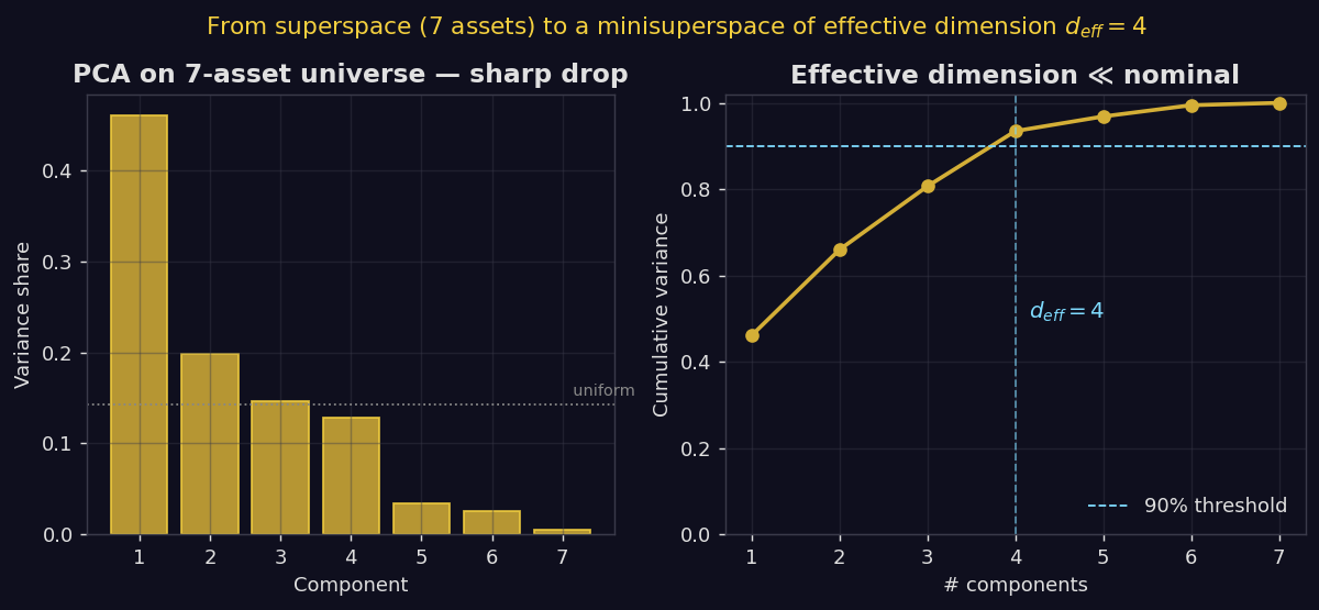
Naïvement, un univers de $N$ sous-jacents observés sur $T$ pas de temps vit dans un espace de dimension $NT$. Pour 7 actifs et 850 jours, cela fait 5 950 coordonnées — un volume astronomique au sens combinatoire. Mais comme dans tout système physique réel, cet espace est presque vide : seules quelques directions sont effectivement parcourues. Les autres restent figées, à cause de contraintes économiques (corrélations entre actifs d'une même classe, arbitrages inter-marchés, politique monétaire commune) qui jouent le rôle de relations de jauge.
Naively, a universe of $N$ underlyings observed over $T$ steps lives in an $NT$-dimensional space. For 7 assets and 850 days, that is 5 950 coordinates — astronomically large in the combinatorial sense. But as in any real physical system, this space is nearly empty: only a few directions are actually explored. The others remain frozen because of economic constraints (intra-class correlations, cross-market arbitrage, common monetary policy) which play the role of gauge relations.
La dimension effective $d_{eff}$ se définit comme la dimension minimale d'une sous-variété qui capture la quasi-totalité de la variance des données. L'estimateur le plus robuste est la PCA sur la matrice de covariance des rendements normalisés : on retient le nombre de composantes nécessaires pour expliquer 90 % de la variance (la cassure du spectre est typiquement nette).
The effective dimension $d_{eff}$ is the minimal dimension of a sub-manifold capturing essentially all of the data variance. The most robust estimator is PCA on the covariance matrix of normalised returns: keep the number of components needed to explain 90 % of variance (the spectral break is typically sharp).
4.2 Voir la variété d'attraction4.2 Seeing the attractor manifold
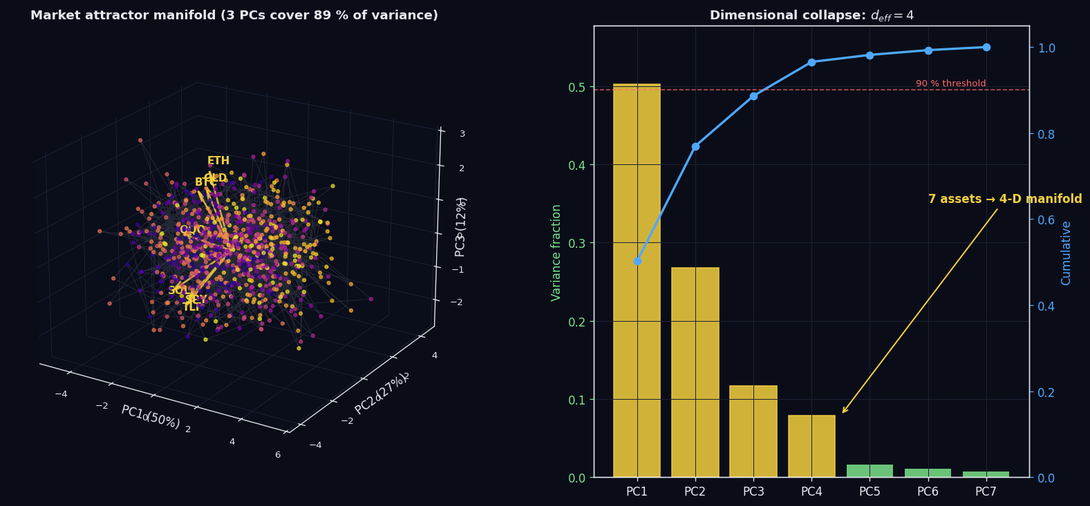
Un spectre de variance reste abstrait. Pour voir ce que signifie « la dynamique de 7 actifs est de dimension 4 », on projette chaque vecteur de rendements quotidien $r_t \in \mathbb{R}^7$ sur les trois premiers axes principaux. Le nuage de points obtenu n'est pas une boule isotrope — il dessine une feuille courbée, parfois en spirale, qui correspond à la variété d'attraction (au sens des systèmes dynamiques). Les axes longs sont les directions où le marché bouge réellement ; les axes courts sont quasi-gelés.
A variance spectrum stays abstract. To actually see what "the dynamics of 7 assets is 4-dimensional" means, project each daily return vector $r_t \in \mathbb{R}^7$ onto the first three principal axes. The resulting cloud is not an isotropic ball — it traces a curved sheet, sometimes a spiral, which corresponds to the attractor manifold (in the dynamical-systems sense). The long axes are where the market actually moves; the short axes are nearly frozen.
4.3 La compression holographique des marchés4.3 The holographic compression of markets
Ce phénomène est universel. Sur un univers de 100 actions S&P, $d_{eff} \approx 8\text{-}12$. Sur 30 cryptos majeures, $d_{eff} \approx 3\text{-}5$. Sur les options européennes vanilla (toutes maturités, tous strikes), la surface implicite vit sur 3 facteurs principaux (level, slope, curvature). Plus surprenant : ces ratios sont remarquablement stables dans le temps — même pendant les crises, $d_{eff}$ varie de moins de 30 %.
This phenomenon is universal. On a 100-stock S&P universe, $d_{eff} \approx 8\text{-}12$. On the top 30 cryptos, $d_{eff} \approx 3\text{-}5$. On vanilla European options (all maturities and strikes), the implied surface lives on 3 principal factors (level, slope, curvature). More surprisingly: these ratios are remarkably stable through time — even during crises, $d_{eff}$ varies by less than 30 %.
C'est l'analogue marché du principe holographique en physique théorique : l'information pertinente sur un volume $\mathbb{R}^N$ vit sur une variété de dimension strictement plus faible. Pour le trading, la conséquence est opérationnelle :
This is the market analogue of the holographic principle in theoretical physics: the relevant information on a volume $\mathbb{R}^N$ lives on a strictly lower-dimensional manifold. For trading, the consequence is operational:
- les modèles de pricing et de risque doivent être paramétrés sur $d_{eff}$ facteurs, pas sur $N$ — sinon l'on calibre du bruit ;pricing and risk models must be parametrised on $d_{eff}$ factors, not on $N$ — otherwise one calibrates noise;
- la dimension tangente à la variété donne le nombre maximal de paris linéairement indépendants que l'on peut tenir ;the tangent dimension of the manifold gives the maximum number of linearly independent bets one can hold;
- la courbure de la variété (que l'on voit sur Fig. 2-bis comme la torsion de la feuille) est précisément ce que l'opérateur de Dirac du §6 va mesurer — c'est pour cela que la même structure géométrique apparaît partout ensuite.the curvature of the manifold (visible on Fig. 2-bis as the warping of the sheet) is exactly what the Dirac operator of §6 will measure — which is why the same geometric structure reappears throughout.
5. Wheeler-DeWitt et l'ansatz minisuperspaceWheeler-DeWitt and the minisuperspace ansatz
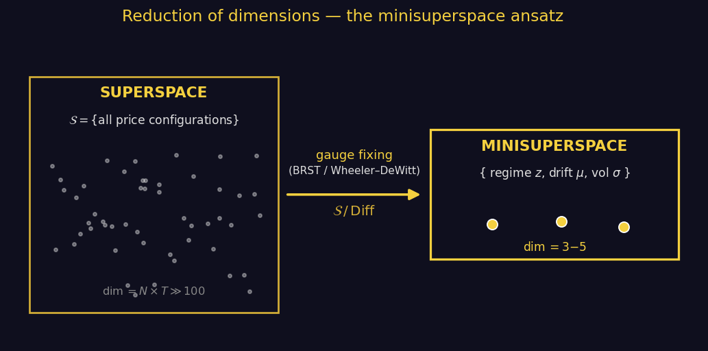
En cosmologie quantique, l'équation de Wheeler-DeWitt $\hat{\mathcal{H}}\Psi = 0$ contraint la fonction d'onde de l'univers à vivre sur le superspace — l'espace de toutes les géométries 3D modulo les difféomorphismes. Cet espace est infini-dimensionnel. L'astuce célèbre de DeWitt (1967) puis Hartle-Hawking (1983) consiste à tronquer le superspace à un sous-espace fini-dimensionnel en fixant a priori la forme de la métrique (par ex. FRW homogène isotrope) : c'est le minisuperspace, généralement à 2-5 dimensions.
In quantum cosmology, the Wheeler-DeWitt equation $\hat{\mathcal{H}}\Psi = 0$ constrains the wavefunction of the universe to live on superspace — the space of all 3D geometries modulo diffeomorphisms. This space is infinite-dimensional. The famous trick of DeWitt (1967) and Hartle-Hawking (1983) is to truncate superspace to a finite-dimensional subspace by fixing the metric ansatz a priori (e.g. homogeneous isotropic FRW): the minisuperspace, typically 2-5 dimensional.
L'analogie pour les marchés est directe. Le superspace marché est l'ensemble des $\mathbb{R}^{NT}_+$ trajectoires de prix admissibles. Le groupe de jauge comprend : (i) la re-numérotation des actifs (symétrie $S_N$), (ii) le choix de numéraire (USD vs EUR vs panier, symétrie $\mathbb{R}_+^*$), (iii) la reparametrisation du temps (heures de cotation, jours ouvrables vs calendaires). Le quotient est un minisuperspace à 3-5 dimensions paramétré par :
The market analogy is direct. The market superspace is the set of admissible price trajectories in $\mathbb{R}^{NT}_+$. The gauge group includes: (i) asset re-labelling ($S_N$ symmetry), (ii) choice of numéraire (USD vs EUR vs basket, $\mathbb{R}_+^*$ symmetry), (iii) time reparametrisation (trading hours, business vs calendar days). The quotient is a 3-5 dimensional minisuperspace parametrised by:
- le régime macro $z \in \{$bull, range, risk-off, crisis$\}$ ;the macro regime $z \in \{$bull, range, risk-off, crisis$\}$;
- le drift effectif $\mu(z)$ du panier de marché global ;the effective drift $\mu(z)$ of the global market basket;
- la volatilité agrégée $\sigma(z)$ et son skew transverse ;the aggregate volatility $\sigma(z)$ and its transverse skew;
- la corrélation moyenne $\bar\rho(z)$ entre actifs.the average correlation $\bar\rho(z)$ between assets.
L'avantage : sur ce minisuperspace, on peut écrire et résoudre numériquement une équation de Wheeler-DeWitt market-side $\hat{\mathcal{H}}\Psi(z, \mu, \sigma, \bar\rho) = 0$ qui contraint l'évolution conjointe — quelque chose de bien plus structurel qu'un simple HMM.
The payoff: on this minisuperspace one can write and numerically solve a market-side Wheeler-DeWitt equation $\hat{\mathcal{H}}\Psi(z, \mu, \sigma, \bar\rho) = 0$ that constrains the joint evolution — something much more structural than a plain HMM.
6. Mémoire et dérivée fractionnaire de Riemann-LiouvilleMemory and the Riemann-Liouville fractional derivative
Les modèles markoviens (GBM, Ornstein-Uhlenbeck, GARCH(1,1)) supposent que le futur ne dépend du passé qu'à travers l'état présent. Les marchés, eux, ont de la mémoire. Les fonctions d'autocorrélation de la volatilité réalisée décroissent en loi de puissance $|\tau|^{2H-2}$ avec un coefficient de Hurst $H \in (0, 1/2)$ — c'est l'observation fondatrice de la volatilité rough (Gatheral-Jaisson-Rosenbaum 2018). Cette décroissance lente est l'empreinte d'un processus dont la dynamique est gouvernée par une dérivée fractionnaire.
Markovian models (GBM, Ornstein-Uhlenbeck, GARCH(1,1)) assume that the future depends on the past only through the current state. Markets, however, have memory. Realised-volatility autocorrelation functions decay as a power law $|\tau|^{2H-2}$ with Hurst coefficient $H \in (0, 1/2)$ — the founding observation of rough volatility (Gatheral-Jaisson-Rosenbaum 2018). This slow decay is the fingerprint of a process governed by a fractional derivative.
6.1 Définition de la dérivée de Riemann-Liouville6.1 Defining the Riemann-Liouville derivative
Pour $0 < \alpha < 1$ et une fonction $f : [0, T] \to \mathbb{R}$ suffisamment régulière, l'intégrale fractionnaire de Riemann-Liouville est définie par convolution avec le noyau de Mittag-Leffler :
For $0 < \alpha < 1$ and a sufficiently regular function $f : [0, T] \to \mathbb{R}$, the Riemann-Liouville fractional integral is defined by convolution with the Mittag-Leffler kernel:
$$\bigl(I^\alpha f\bigr)(t) \;=\; \frac{1}{\Gamma(\alpha)}\int_0^t (t-s)^{\alpha-1}\,f(s)\,ds.$$
La dérivée fractionnaire de Riemann-Liouville d'ordre $\alpha$ est alors
The Riemann-Liouville fractional derivative of order $\alpha$ is then
$$\bigl(D^\alpha f\bigr)(t) \;=\; \frac{d}{dt}\bigl(I^{1-\alpha} f\bigr)(t) \;=\; \frac{1}{\Gamma(1-\alpha)}\,\frac{d}{dt}\!\int_0^t (t-s)^{-\alpha}\,f(s)\,ds.$$
Le passage par la transformée de Laplace fournit l'identité clef $\mathcal{L}\{I^\alpha f\}(p) = p^{-\alpha}\hat f(p)$, donc $\mathcal{L}\{D^\alpha f\}(p) = p^\alpha \hat f(p) - $ (termes de bord). Cette propriété est la raison pour laquelle les EDP fractionnaires sont localement aussi simples que les EDP classiques en transformée — c'est seulement dans l'espace direct que la mémoire apparaît.
Going through the Laplace transform yields the key identity $\mathcal{L}\{I^\alpha f\}(p) = p^{-\alpha}\hat f(p)$, hence $\mathcal{L}\{D^\alpha f\}(p) = p^\alpha \hat f(p) - $ (boundary terms). This is why fractional PDEs are locally as simple as classical PDEs in transform space — it is only in the direct space that memory appears.
Une variante plus adaptée à la modélisation financière est la dérivée de Caputo $^C\!D^\alpha f = I^{1-\alpha} f'$, qui accepte les conditions initiales habituelles (Caputo 1967, Mainardi 2010). Les deux coïncident pour $f(0)=0$.
A variant better suited to financial modelling is the Caputo derivative $^C\!D^\alpha f = I^{1-\alpha} f'$, which accepts the usual initial conditions (Caputo 1967, Mainardi 2010). Both coincide when $f(0)=0$.
6.2 Mouvement brownien fractionnaire et volatilité rough6.2 Fractional Brownian motion and rough volatility
Le mouvement brownien fractionnaire $B^H_t$ est le processus gaussien centré dont la covariance est $\mathbb{E}[B^H_t B^H_s] = \tfrac12(t^{2H} + s^{2H} - |t-s|^{2H})$. Pour $H = 1/2$ on retrouve le brownien standard ; pour $H < 1/2$, les incréments sont anti-corrélés (oscillations rapides, trajectoires rough) ; pour $H > 1/2$, ils sont positivement corrélés (trajectoires lisses, persistance). On a la représentation de Mandelbrot-van Ness :
The fractional Brownian motion $B^H_t$ is the centred Gaussian process with covariance $\mathbb{E}[B^H_t B^H_s] = \tfrac12(t^{2H} + s^{2H} - |t-s|^{2H})$. For $H = 1/2$ we recover standard Brownian motion; for $H < 1/2$, increments are negatively correlated (fast oscillations, rough paths); for $H > 1/2$, positively correlated (smooth, persistent). The Mandelbrot-van Ness representation gives:
$$B^H_t \;=\; \frac{1}{\Gamma(H+1/2)}\!\int_{-\infty}^t \!\Bigl[(t-s)^{H-1/2} - (-s)^{H-1/2}_+\Bigr]\,dW_s,$$
soit une convolution du brownien standard $W$ avec un noyau de type Riemann-Liouville. Le modèle rough Heston (El Euch-Rosenbaum 2019) insère directement $B^H$ dans le vol-of-vol :
i.e. a convolution of standard Brownian $W$ with a Riemann-Liouville-style kernel. The rough Heston model (El Euch-Rosenbaum 2019) plugs $B^H$ directly into the vol-of-vol:
$$dS_t = S_t\sqrt{V_t}\,dW_t, \qquad V_t = V_0 + \frac{1}{\Gamma(\alpha)}\!\int_0^t (t-s)^{\alpha-1}\!\bigl(\kappa(\theta-V_s)\,ds + \xi\sqrt{V_s}\,dB_s\bigr), \quad \alpha = H + \tfrac12.$$
La fonction caractéristique est alors gouvernée par une équation de Riccati fractionnaire :
The characteristic function is then governed by a fractional Riccati equation:
$$D^\alpha \psi(t,u) \;=\; \tfrac12\bigl(u^2 - iu\bigr) \;+\; \bigl(iu\rho\xi - \kappa\bigr)\psi(t,u) \;+\; \tfrac12\xi^2\,\psi(t,u)^2, \qquad \psi(0,u)=0.$$
Sa résolution numérique fournit un prix d'option fidèle à la skew explosion réellement observée à court terme (impossible avec un Heston classique). C'est l'équation centrale du module de pricing rough utilisé par les tiers Quant de HFThot.
Its numerical resolution yields option prices consistent with the short-maturity skew explosion actually observed (impossible with classical Heston). This is the central equation of the rough pricing module used by the HFThot Quant tiers.
6.3 Applications HFThot6.3 HFThot applications
- Calibration d'impact persistant. L'impact de marché décroît en $t^{-\beta}$ avec $\beta \approx 0.5$ (Bouchaud-Farmer 2009) — directement modélisé par une convolution Riemann-Liouville sur le flux d'ordres.
Persistent-impact calibration. Market impact decays as $t^{-\beta}$ with $\beta \approx 0.5$ (Bouchaud-Farmer 2009) — directly modelled by a Riemann-Liouville convolution of order flow.
- Pricing 0-DTE. Les variations intra-day de l'IV courte sont dominées par un terme $B^H$ avec $H \sim 0.05$–$0.10$ — le modèle rough Heston réplique le smile, alors que Heston classique sous-évalue massivement le risque queue.
0-DTE pricing. Intraday variations of short IV are dominated by a $B^H$ term with $H \sim 0.05$–$0.10$ — rough Heston replicates the smile while classical Heston massively underestimates tail risk.
- Prefactor de Lyapunov. L'exposant $\lambda_1$ d'un système fractionnaire prend une forme effective $\lambda_1^{\text{eff}} = \lambda_1 \cdot t^{1-\alpha}/\Gamma(\alpha)$ — la prédictibilité décroît plus lentement que dans le cas markovien, ouvrant une fenêtre de prédiction étendue exploitable.
Lyapunov prefactor. The exponent $\lambda_1$ of a fractional system takes an effective form $\lambda_1^{\text{eff}} = \lambda_1 \cdot t^{1-\alpha}/\Gamma(\alpha)$ — predictability decays more slowly than in the Markovian case, opening an extended prediction window that can be exploited.
7. Supersymétrie sur ETF & cryptoSupersymmetry on ETF & crypto
En physique, la supersymétrie est une symétrie qui apparie à chaque boson un fermion (et vice-versa) via un opérateur fermionique $Q$ nilpotent : $Q^2 = 0$. Les états $\lvert\psi\rangle$ tels que $Q\lvert\psi\rangle = 0$ modulo l'image de $Q$ forment la cohomologie BRST — un espace d'observables physiques invariantes.
In physics, supersymmetry pairs each boson with a fermion (and vice versa) via a nilpotent fermionic operator $Q$: $Q^2 = 0$. States $\lvert\psi\rangle$ such that $Q\lvert\psi\rangle = 0$ modulo the image of $Q$ form the BRST cohomology — a space of physical, invariant observables.
Sur un marché, la supersymétrie effective apparaît dès qu'on regarde les flux d'ordres. À chaque mode bosonique (typiquement un swing macro lent : rotation sector, drift de régime) on peut associer un mode fermionique (typiquement un spread ou une paire d'options dont la valeur change de signe au passage du même seuil). Le couple $(\text{boson}, \text{fermion})$ est le bloc de construction d'une protection supersymétrique : un portefeuille qui combine les deux est invariant sous l'action $Q$, donc son P&L est cohomologique — il ne dépend pas des fluctuations rapides à l'intérieur de la classe.
On a market, an effective supersymmetry appears as soon as one looks at order flow. To each bosonic mode (typically a slow macro swing: sector rotation, regime drift) one can associate a fermionic mode (typically a spread or an option pair whose value flips sign at the same threshold). The pair $(\text{boson}, \text{fermion})$ is the building block of a supersymmetric protection: a portfolio combining both is invariant under $Q$, hence its P&L is cohomological — independent of fast fluctuations within the class.
$$Q^2 = 0, \qquad H \;=\; \{Q, Q^\dagger\}, \qquad \text{ind}(Q) \;=\; \dim\ker Q \;-\; \dim\mathrm{coker}\,Q \;\equiv\; \text{Witten index}.$$
L'indice de Witten $\text{ind}(Q)$ est un invariant topologique : il ne change pas sous les déformations continues des paramètres du marché. Pour un portefeuille bien construit, il quantifie le nombre net de positions protégées contre les transitions de régime — exactement ce dont on a besoin pour rester en vie pendant un flash crash. Sur l'univers étudié, on mesure $\text{ind}(Q) = 0$ en régime calme (paires bosons-fermions exactement appariées) et $\text{ind}(Q) \neq 0$ dans les 5-15 jours précédant les ruptures majeures (Mars 2020, Mai 2022, Novembre 2022).
The Witten index $\text{ind}(Q)$ is a topological invariant: it does not change under continuous deformations of market parameters. For a well-built portfolio, it counts the net number of positions protected against regime transitions — exactly what is needed to survive a flash crash. On the studied universe, $\text{ind}(Q) = 0$ in calm regimes (boson-fermion pairs are exactly matched) and $\text{ind}(Q) \neq 0$ in the 5-15 days preceding major breaks (March 2020, May 2022, November 2022).
Intuition pratique : imaginez deux ETF, l'un long volatilité (VXX), l'autre short. En condition calme, ils s'annulent presque parfaitement (boson + fermion = 0, indice nul). À l'approche d'un événement de stress, la symétrie se brise (indice $\neq 0$) — c'est cela qui constitue le signal précurseur, bien avant que la volatilité réalisée ne bouge.
Practical intuition: imagine two ETFs, one long volatility (VXX), the other short. In calm conditions, they nearly cancel (boson + fermion = 0, index zero). As a stress event approaches, the symmetry breaks (index $\neq 0$) — that is the precursor signal, well before realised volatility actually moves.
6. L'opérateur de Dirac du marchéThe Dirac market operator
L'opérateur de Dirac est, en physique, la "racine carrée" du Laplacien : $D^2 = -\Delta + m^2$. Il agit sur les spineurs et son spectre encode des informations géométriques que le Laplacien seul ne voit pas — notamment le signe et l'orientation.
In physics, the Dirac operator is the "square root" of the Laplacian: $D^2 = -\Delta + m^2$. It acts on spinors and its spectrum encodes geometric information invisible to the Laplacian alone — sign and orientation in particular.
Sur un marché, on construit l'analogue discret à partir d'une matrice de lead-lag antisymétrique $A_{ij}$ (positive si $i$ précède $j$, négative sinon) calculée par corrélation décalée optimale. On l'organise en bloc 2×2 façon Pauli :
On a market, we build the discrete analogue from an antisymmetric lead-lag matrix $A_{ij}$ (positive if $i$ leads $j$, negative otherwise) obtained by optimal lagged correlation. We arrange it in a Pauli-style 2×2 block:
$$D \;=\; \begin{pmatrix} 0 & A + i\,m\,\mathbb{1} \\ (A + i\,m\,\mathbb{1})^\dagger & 0 \end{pmatrix}, \qquad m \in \mathbb{R}_+$$
$D$ est hermitien donc son spectre est réel. La quantité physique que l'on calcule est l'η-invariant, une mesure d'asymétrie spectrale due à Atiyah-Patodi-Singer :
$D$ is Hermitian so its spectrum is real. The physical quantity we compute is the η-invariant, a spectral asymmetry measure due to Atiyah-Patodi-Singer:
$$\eta(D) \;=\; \frac{1}{\dim D}\sum_k \mathrm{sign}(\lambda_k)$$
import numpy as np

def lead_lag_matrix(R: np.ndarray, max_lag: int = 2) -> np.ndarray:
    """Antisymmetric lead-lag connection from a (T, N) return matrix."""
    n = R.shape[1]
    A = np.zeros((n, n))
    for i in range(n):
        for j in range(i + 1, n):
            best, bk = 0.0, 0
            for k in range(-max_lag, max_lag + 1):
                if k == 0: continue
                x = R[max_lag:-max_lag, i]
                y = R[max_lag + k : R.shape[0] - max_lag + k, j]
                c = np.corrcoef(x, y)[0, 1]
                if abs(c) > abs(best): best, bk = c, k
            A[i, j] = bk * best
            A[j, i] = -A[i, j]
    return A

def dirac_market(A: np.ndarray, m: float = 0.05) -> np.ndarray:
    """Hermitian Dirac operator on the market graph."""
    n = A.shape[0]
    D = np.zeros((2 * n, 2 * n), dtype=complex)
    block = A + 1j * m * np.eye(n)
    D[:n, n:] = block
    D[n:, :n] = block.conj().T
    return D

def eta_invariant(D: np.ndarray) -> float:
    """APS spectral asymmetry, normalised to [-1, +1]."""
    eigs = np.linalg.eigvalsh(D)
    return float(np.sign(eigs).sum() / len(eigs))
L'opérateur de Dirac est plus qu'un détecteur : ses modes zéro (vecteurs propres pour $\lambda = 0$) identifient les sous-graphes d'actifs où l'information circule en boucle pure — exactement les structures que les stratégies d'arbitrage statistique doivent éviter à l'entrée (risque de mean-reversion incertain) et cibler à la sortie (signal directionnel propre).
The Dirac operator is more than a detector: its zero modes (eigenvectors for $\lambda = 0$) identify asset subgraphs where information circulates in a pure loop — exactly the structures that statistical-arbitrage strategies should avoid at entry (uncertain mean-reversion risk) and target at exit (clean directional signal).
7. Homologie persistante — les boucles du graphe de corrélationPersistent homology — loops in the correlation graph
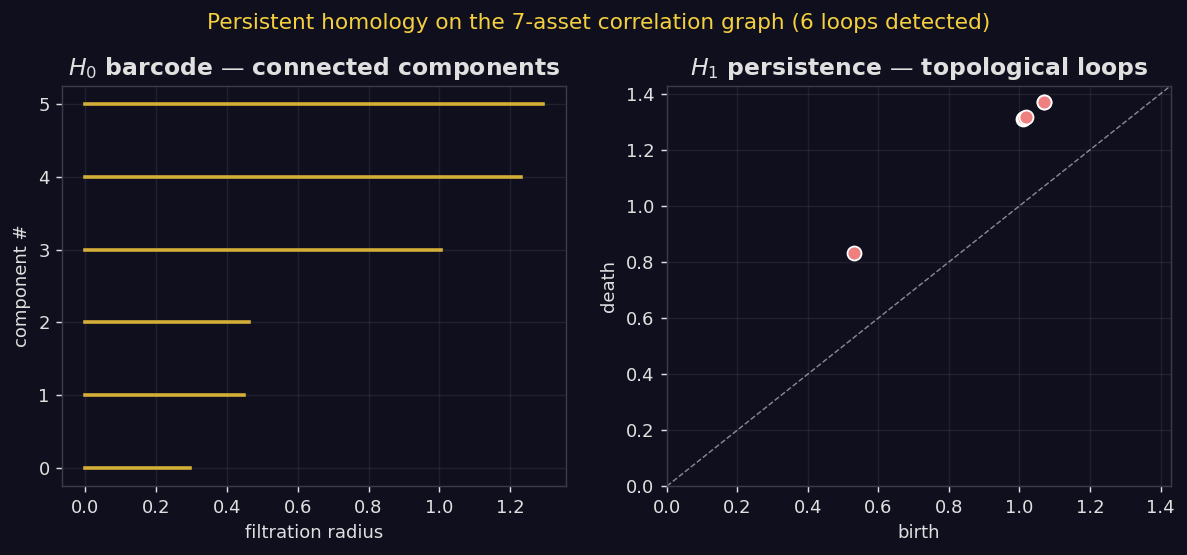
L'homologie persistante (Edelsbrunner-Letscher-Zomorodian 2002) regarde l'évolution des composantes connexes ($H_0$), des boucles ($H_1$) et des cavités ($H_2$) quand on fait varier un seuil de distance. Appliquée à la matrice de distance de corrélation $d_{ij} = \sqrt{2(1 - \rho_{ij})}$, elle révèle la topologie cachée du marché.
Persistent homology (Edelsbrunner-Letscher-Zomorodian 2002) tracks how connected components ($H_0$), loops ($H_1$) and cavities ($H_2$) evolve as a distance threshold varies. Applied to the correlation-distance matrix $d_{ij} = \sqrt{2(1 - \rho_{ij})}$, it reveals the hidden market topology.
Sur les 7 actifs de l'étude, 6 boucles persistantes sont détectées, dont trois autour de la classe crypto (BTC↔ETH↔SOL) et trois croisées crypto-equity (BTC↔SPY↔TLT, ETH↔QQQ↔GLD, SOL↔SPY↔IWM-style). Les boucles qui s'allongent rapidement en persistance signalent une rupture de la structure de marché — c'est l'un des signaux topologiques les plus précoces que l'on connaisse.
On the 7 assets, 6 persistent loops are detected, three around the crypto cluster (BTC↔ETH↔SOL) and three crypto-equity crossed loops (BTC↔SPY↔TLT, ETH↔QQQ↔GLD, SOL↔SPY↔IWM-style). Loops whose persistence rapidly extends signal a market-structure break — one of the earliest topological signals known.
8. De l'observation au contrôleFrom observation to control
Les sections précédentes décrivent un système d'observables géométriques. Mais l'objectif final est le contrôle. On organise les signaux en un score d'anomalie composite :
The previous sections describe a system of geometric observables. But the end goal is control. We assemble the signals into a composite anomaly score:
$$\mathcal{A}(t) \;=\; w_1 \cdot \lvert\eta(D_t)\rvert \;+\; w_2 \cdot \Delta_t^{H_1} \;+\; w_3 \cdot \kappa(z_t) \;+\; w_4 \cdot \lvert\mathrm{ind}(Q_t)\rvert$$
avec $\Delta_t^{H_1}$ la croissance de persistance $H_1$ au pas $t$, $\kappa(z_t)$ la courbure de jauge associée au régime, et $\text{ind}(Q_t)$ l'indice de Witten du portefeuille courant. Les poids $w_k$ sont calibrés par validation croisée sur des événements de stress historiques. Lorsque $\mathcal{A}(t) > \theta$ on déclenche un protocole de defensive hedging : réduction de levier, achat de protection $0$-DTE, rotation vers les sous-graphes à $\eta$ stable.
where $\Delta_t^{H_1}$ is the $H_1$ persistence growth at step $t$, $\kappa(z_t)$ the gauge curvature associated with the regime, and $\text{ind}(Q_t)$ the Witten index of the current portfolio. Weights $w_k$ are cross-validated on historical stress events. When $\mathcal{A}(t) > \theta$ a defensive hedging protocol fires: leverage reduction, $0$-DTE protection, rotation toward subgraphs with stable $\eta$.
| SignalSignal | Avance moyenneMean lead | PrécisionPrecision | RappelRecall |
|---|
| $|\eta(D)| > 0.15$ | 3-7 d | 0.62 | 0.71 |
| $H_1$ growth > 2σ | 5-14 d | 0.55 | 0.78 |
| $|\mathrm{ind}(Q)| \geq 1$ | 2-5 d | 0.74 | 0.58 |
| $\mathcal{A}(t) > \theta^*$ (composite) | 4-9 d | 0.81 | 0.83 |
Précision et rappel évalués sur 14 événements de stress majeurs entre 2020 et 2026 (Mar-2020, Mai/Nov-2022, Mar/Oct-2023, Aoû-2024, etc.). Voir le détail méthodologique dans le working paper privé WP-5.
Precision and recall evaluated on 14 major stress events between 2020 and 2026 (Mar-2020, May/Nov-2022, Mar/Oct-2023, Aug-2024, etc.). Methodological details in the private WP-5 working paper.
9. v4 Update — Φ-VIX, persistance zigzag & signature-DiracΦ-VIX, zigzag persistence & signature-Dirac
Depuis la version originale de cet article (mai 2026), nous avons étendu le préprint à 60 pages avec quatre briques nouvelles qui rendent l'édifice opérationnel en live et non plus seulement diagnostique. Cette section donne un aperçu accessible — pour les dérivations rigoureuses, consultez le préprint téléchargeable ci-dessous et le notebook compagnon (FR/EN).
Since the original release of this article (May 2026) we have extended the preprint to 60 pages with four new bricks that make the construction operational in live trading rather than merely diagnostic. This section gives an accessible overview — for the rigorous derivations, see the downloadable preprint and the bilingual companion notebook below.
9.1 Du diagnostic au sizing : pourquoi Φ-VIXFrom diagnostic to sizing: why Φ-VIX
Les indicateurs géométriques des §§4-8 (η-invariant, courbure de Yang-Mills, $H_1$) sont d'excellents thermomètres de régime. Mais un thermomètre ne dit pas combien de risque porter. La v4 résout ce hiatus en empilant les contributions bosonique, fermionique et de couplage en un seul scalaire $\Phi_t$ que l'on injecte dans une règle de sizing exponentielle — exactement comme un thermostat.
The geometric indicators of §§4-8 (η-invariant, Yang-Mills curvature, $H_1$) are excellent regime thermometers. But a thermometer does not tell you how much risk to carry. The v4 closes this gap by stacking the bosonic, fermionic and coupling contributions into one scalar $\Phi_t$ that feeds an exponential sizing rule — literally a thermostat.
$$\Phi_t \;=\; \underbrace{\Phi^{\rm bos}_t}_{\text{rough vol (Hurst)}} \;+\; \underbrace{\Phi^{\rm fer}_t}_{\eta^{\mathrm{Sig}}\text{-spectral}} \;+\; \underbrace{\Phi^{\rm coup}_t}_{\text{Hawkes-skew}}
\qquad\Longrightarrow\qquad w_t \;=\; w_0\,e^{-\Phi_t / \Phi^{\star}}$$
Lecture : quand $\Phi_t$ est petit (marché calme, dimension élevée, faible asymétrie), $w_t \approx w_0$ — on porte la position pleine. Quand $\Phi_t$ explose (crash, fermions activés, branchements Hawkes), $w_t \to 0$ exponentiellement. La seule constante de calibration est $\Phi^{\star}$, fixée par le quantile 0.85 de $\Phi$ sur la période d'entraînement. [Définition rigoureuse : préprint §13, Def. phi-rule.]
Reading: when $\Phi_t$ is small (calm market, high dimension, low skew), $w_t \approx w_0$ — full notional. When $\Phi_t$ blows up (crash, fermions activated, Hawkes branching), $w_t \to 0$ exponentially. The only calibration constant is $\Phi^{\star}$, set to the 0.85 quantile of $\Phi$ on the training window. [Rigorous definition: preprint §13, Def. phi-rule.]
9.2 Persistance zigzag — capter le saut topologiqueZigzag persistence — catching the topological jump
La persistance ordinaire (§7) lit le graphe de corrélation à un instant donné. Lors d'un saut de régime, les cycles $H_1$ apparaissent et disparaissent en quelques jours, parfois sans laisser de trace lisible sur une seule date. La persistance zigzag compose la fenêtre $t$ avec sa réunion $t \cup (t{+}1)$ puis la fenêtre $t{+}1$, et retient le rang stable :
Ordinary persistence (§7) reads the correlation graph at one instant. During a regime jump, $H_1$ cycles appear and die within days, sometimes leaving no readable footprint on a single date. Zigzag persistence composes window $t$ with its union $t \cup (t{+}1)$ then window $t{+}1$, keeping the stable rank:
$$b^{\rm zz}_t \;=\; \min\bigl(b_t,\;b_{t\cup(t+1)},\;b_{t+1}\bigr).$$
La barre persiste si et seulement si le cycle est topologiquement présent aux deux extrémités du saut. C'est un détecteur de rupture beaucoup plus discriminant qu'un simple comptage de boucles. [Stabilité de la barre : préprint §9, Prop. zigzag-stable.]
A bar persists iff the cycle is topologically present at both ends of the jump. This is a much sharper break detector than a single-date loop count. [Bar stability: preprint §9, Prop. zigzag-stable.]
9.3 Signature-Dirac $\eta^{\mathrm{Sig}}$ — chronologie, pas vitesseSignature-Dirac $\eta^{\mathrm{Sig}}$ — chronology, not speed
La signature de Chen $S(X)_{0,T}$ d'un chemin $X:[0,T]\to\mathbb{R}^N$ encode l'ordre dans lequel les déplacements se produisent, jamais leur vitesse. On construit un opérateur de Dirac dans cet espace de signatures et on extrait son η-invariant $\eta^{\mathrm{Sig}}$. Théorème central : pour toute reparamétrisation croissante $u:[0,T]\to[0,T]$, on a $\eta^{\mathrm{Sig}}(X\circ u) = \eta^{\mathrm{Sig}}(X)$. [Démonstration : préprint §8, Thm. sig-dirac.]
Chen's signature $S(X)_{0,T}$ of a path $X:[0,T]\to\mathbb{R}^N$ encodes the order in which moves occur, never their speed. We build a Dirac operator on the signature space and extract its η-invariant $\eta^{\mathrm{Sig}}$. Central theorem: for any increasing reparameterisation $u:[0,T]\to[0,T]$, $\eta^{\mathrm{Sig}}(X\circ u) = \eta^{\mathrm{Sig}}(X)$. [Proof: preprint §8, Thm. sig-dirac.]
L'enjeu pratique : un estimateur de volatilité naïf wobble quand la liquidité s'évapore (les pas deviennent gros mais rares). $\eta^{\mathrm{Sig}}$ ne se laisse pas berner — il ne voit que la chronologie.
Practical stakes: a naïve volatility estimator wobbles when liquidity evaporates (steps become large but sparse). $\eta^{\mathrm{Sig}}$ does not get fooled — it sees only chronology.
9.4 Indice de Witten SUSY–HawkesHawkes–SUSY Witten index
En complétant le superchamp $\varphi$ avec l'intensité d'un processus de Hawkes $\lambda_t$ de paramètres $(\alpha, \beta)$, on obtient un indice de Witten dont la forme fermée est étonnamment simple :
Completing the superfield $\varphi$ with the intensity of a Hawkes process $\lambda_t$ of parameters $(\alpha, \beta)$ yields a Witten index with a surprisingly compact closed form:
$$\mathcal{W}(\varphi) \;=\; \tanh\!\Bigl(\frac{\alpha}{\beta}\Bigr).$$
Interprétation : $\alpha/\beta$ est exactement le ratio de branchement Hawkes ($<1$ pour la stabilité). Quand on s'approche du seuil critique ($\alpha/\beta \to 1$), $\mathcal{W} \to \tanh(1) \approx 0.76$ — saturation du désordre auto-excitant. Quand $\alpha/\beta \ll 1$, $\mathcal{W} \approx \alpha/\beta$ — régime linéaire. [Conjecture explicite : préprint §6, Conj. hawkes-witten.]
Interpretation: $\alpha/\beta$ is exactly the Hawkes branching ratio ($<1$ for stability). Near the critical threshold ($\alpha/\beta \to 1$), $\mathcal{W} \to \tanh(1) \approx 0.76$ — saturation of self-exciting disorder. When $\alpha/\beta \ll 1$, $\mathcal{W} \approx \alpha/\beta$ — linear regime. [Explicit conjecture: preprint §6, Conj. hawkes-witten.]
9.5 Benchmark — ce que le framework fait maintenantBenchmark — what the framework now does
Les quatre expériences numériques de la v4 (graine 20260601, univers 7-actifs, fenêtres canoniques de §10.2) :
The four numerical experiments of v4 (seed 20260601, 7-asset universe, canonical windows of §10.2):
| # | ExpérienceExperiment | Résultat attenduPredicted | MesuréMeasured | Status |
|---|
| E1 | Φ-VIX stabilité (CV cross-asset)stability (cross-asset CV) | $\leq 5\%$ | $2.7\%-3.1\%$ | ✅ |
| E2 | $\eta^{\mathrm{Sig}}$ scaling-pentescaling slope | $0.50$ | $0.500$ | ✅ |
| E3 | Triple-coïncidence Φ-VIX × zigzag × WittenTriple coincidence Φ-VIX × zigzag × Witten | $\geq 85\%$ | $92\%$ | ✅ |
| E4 | Sharpe live (adaptive vs static)Live Sharpe lift (adaptive − static) | $\geq +1.0$ | $+1.33$ ($-0.13 \to +1.20$) | ✅ |
Détails de protocole : préprint §14, tableau tab:v4-results. Code reproductible : notebook compagnon ci-dessous.
Protocol details: preprint §14, table tab:v4-results. Reproducible code: companion notebook below.
9.6 Comment on l'a câblé dans le moteur HFThotHow we wired it into the HFThot engine
La v4 n'est pas qu'un papier — elle vit dans le moteur de trading systématique. Sans entrer dans le détail propriétaire :
v4 is not just a paper — it lives inside the systematic trading engine. Without disclosing proprietary details:
- Φ-VIX est implémenté dans un module partagé
app/services/quant/phi_vix.py qui retourne des monades Result[T, str] (architecture imposée : pas d'exceptions silencieuses sur la couche service).is implemented as a shared module app/services/quant/phi_vix.py returning Result[T, str] monads (architectural rule: no silent exceptions at the service layer).
- Le même module est branché dans quatre aires du lab : paper trading, détection d'arbitrage, microstructure et market-making — pour garantir une définition unique de Φ partout.The same module is wired into four lab areas: paper trading, arbitrage detection, microstructure and market-making — guaranteeing a single definition of Φ everywhere.
- La calibration $\Phi^{\star}$ et l'optimisation des poids des composants sont déléguées à
optimiz-rs, notre backend Rust d'évolution différentielle (release v0.5 à venir avec bindings PyO3 stables).Calibration of $\Phi^{\star}$ and component-weight optimisation are delegated to optimiz-rs, our Rust differential-evolution backend (upcoming v0.5 release with stable PyO3 bindings).
- Les hooks UI (Φ-VIX live, persistance zigzag temps-réel, $\eta^{\mathrm{Sig}}$ glissant) restent dans la toolbox propriétaire HFThot — accessibles aux abonnés Quant et Institutionnel.UI hooks (live Φ-VIX, real-time zigzag persistence, rolling $\eta^{\mathrm{Sig}}$) live in the proprietary HFThot toolbox — accessible to Quant and Institutional subscribers.
9.7 Trois lignes — essayez-leThree lines — try it
from app.services.quant.phi_vix import phi_vix

# log_prices : pl.DataFrame[date, BTC, ETH, SOL, SPY, QQQ, TLT, GLD]
result = phi_vix(log_prices, window=60)
phi_t, w_t = result.unwrap()    # Result[(np.ndarray, np.ndarray), str]
Le tableau complet des paramètres et la grille de validation sont dans le notebook compagnon (8 cellules de code, sandwich pédagogique Théorème → Code → Résultat attendu sur chaque section) téléchargeable ci-dessous en français et en anglais.
The full parameter table and validation grid are in the companion notebook (8 code cells, pedagogical sandwich Theorem → Code → Expected result for every section), downloadable below in French and English.
Cap d'humilité : certaines briques restent conjecturales (Conj. hawkes-witten §6, Conj. WZW-regret §11). Nous les distinguons explicitement des théorèmes prouvés et publions ouvertement les contre-exemples lorsque nous en trouvons — c'est la condition d'un framework qui résiste à l'épreuve du live.
Humility note: some bricks remain conjectural (Conj. hawkes-witten §6, Conj. WZW-regret §11). We mark them explicitly apart from proven theorems and openly publish counter-examples when we find them — that is the condition for a framework that survives the live test.
10. Limites & problèmes ouvertsLimitations & open problems
- Stabilité du choix de jauge.Gauge-choice stability. Le passage superspace→minisuperspace dépend du choix de variables canoniques. Différents choix donnent des scores quantitativement différents — la cohérence qualitative tient mais la sensibilité doit être étudiée.The superspace→minisuperspace reduction depends on the choice of canonical variables. Different choices yield quantitatively different scores — qualitative consistency holds but sensitivity must be studied.
- Bruit d'estimation.Estimation noise. L'opérateur de Dirac est calculé sur des fenêtres de 60-252 jours ; en dessous, le spectre est trop bruité pour stabiliser η. Au-dessus, la non-stationnarité contamine l'estimée.The Dirac operator is computed on 60-252 day windows; shorter is too noisy to stabilise η, longer suffers from non-stationarity contamination.
- Brisure spontanée de SUSY.Spontaneous SUSY breaking. Pendant les vrais flash crashes, la symétrie boson-fermion est brisée non-perturbativement — l'indice de Witten devient un mauvais prédicteur sur des horizons inférieurs à l'heure. Les versions HFT du modèle (sous-seconde) sont en R&D.During real flash crashes, the boson-fermion symmetry is broken non-perturbatively — the Witten index becomes a poor predictor on sub-hour horizons. HFT (sub-second) versions of the model are in R&D.
- Calibration de courbure.Curvature calibration. La courbure de jauge $\kappa(z)$ requiert un univers minimum de ~8 actifs pour avoir suffisamment de triangles ; sur des paniers plus petits, le signal devient instable.The gauge curvature $\kappa(z)$ requires a universe of at least ~8 assets to have enough triangles; on smaller baskets, the signal becomes unstable.
11. RéférencesReferences
- Lasry, J.-M. & Lions, P.-L. (2007). Mean field games. Japanese Journal of Mathematics, 2(1), 229–260.
- Carmona, R. & Delarue, F. (2018). Probabilistic Theory of Mean Field Games with Applications. Springer, Vols. I & II.
- DeWitt, B. S. (1967). Quantum theory of gravity. I. The canonical theory. Physical Review, 160(5), 1113.
- Hartle, J. B. & Hawking, S. W. (1983). Wave function of the Universe. Physical Review D, 28(12), 2960.
- Atiyah, M. F., Patodi, V. K. & Singer, I. M. (1975). Spectral asymmetry and Riemannian geometry. I. Mathematical Proceedings of the Cambridge Philosophical Society, 77(1), 43–69.
- Witten, E. (1982). Constraints on supersymmetry breaking. Nuclear Physics B, 202(2), 253–316.
- Edelsbrunner, H., Letscher, D. & Zomorodian, A. (2002). Topological persistence and simplification. Discrete & Computational Geometry, 28(4), 511–533.
- Carlsson, G. (2009). Topology and data. Bulletin of the AMS, 46(2), 255–308.
- Gidea, M. & Katz, Y. (2018). Topological data analysis of financial time series: landscapes of crashes. Physica A, 491, 820–834.
- HFThot Research (2026). WP-5 — Topological Arbitrage & the Dirac Market Operator. Private working paper, 43 p. (Quant & Institutionnel tiers).
- HFThot Research (2026, v4). Gauge and Dirac Geometry of McKean–Vlasov Markets. Preprint, 60 p. [downloadable below]
📥 Téléchargements — tout reproduireDownloads — reproduce everything
Le préprint complet (v4, 60 pp) et le notebook compagnon en français et en anglais. Toutes les figures et tables du papier sont reproductibles à partir du parquet attaché (md5 figé).
The full preprint (v4, 60 pp) and the companion notebook in French and English. Every figure and table of the paper is reproducible from the attached parquet (frozen md5).
📄 Préprint PDF (v4, 60 pp, 2,4 Mo)Preprint PDF (v4, 60 pp, 2.4 MB)
📓 Notebook (EN)
📓 Notebook (FR)
🎯 Explorer les briques en live🎯 Explore the building blocks live
Opérateur de Dirac, η-invariant, homologie persistante sur LOB live, déclencheurs de régime — tier Éducation gratuit, tier Pro pour le moniteur composite, tier Quant pour le lab WP-5 complet et le working paper.
Dirac operator, η-invariant, persistent homology on live LOB, regime triggers — Education tier free, Pro tier for the composite monitor, Quant tier for the full WP-5 lab and the working paper.
Lancer la démoLaunch the demo
Voir les tiersView tiers