1. Faits stylisés de la microstructure cross-assetStylised facts of cross-asset microstructure

Trois régularités empiriques guident toute modélisation de PnL court-terme au niveau portefeuille: Three empirical regularities guide any portfolio-level short-term PnL modelling:

1. Co-mouvement & lead-lag. Sur les actifs liquides (BTC/ETH, équités sœurs, paires FX), la corrélation des log-returns à l'échelle 1 s est typiquement > 0.4 et présente un lead de 50–500 ms du marché le plus profond vers les autres (Hayashi-Yoshida, 2005). For liquid assets (BTC/ETH, peer equities, FX pairs), 1-second log-return correlations are typically > 0.4 and exhibit a 50–500 ms lead of the deepest market over the others (Hayashi-Yoshida, 2005).
2. Mean-reversion & spreads cointégrés. Le spread normalisé entre deux actifs corrélés est typiquement Ornstein-Uhlenbeck à des demi-vies de quelques minutes à quelques heures — c'est exactement la justification du cadre OU multi-actif. The normalised spread between two correlated assets is typically Ornstein-Uhlenbeck with half-lives ranging from minutes to hours — precisely the justification for the multi-asset OU framework.
3. Impact concave et auto-corrélé. L'impact temporaire reste bien approximé par un terme quadratique $\frac12 v^\top \eta v$ tant que la vitesse de trading reste inférieure à $\sim 5\%$ du volume de la barre. Temporary impact remains well approximated by a quadratic term $\frac12 v^\top \eta v$ as long as trading speed stays below $\sim 5\%$ of the bar volume.

2. Dynamiques OU multi-actifMulti-asset OU dynamics

Soit $S_t \in \mathbb{R}^d$ le vecteur des $d$ mid-prices d'un panier. Bergault, Drissi & Guéant (2022) supposent la dynamique multivariée: Let $S_t \in \mathbb{R}^d$ be the vector of $d$ basket mid-prices. Bergault, Drissi & Guéant (2022) assume the multivariate dynamics:

avec $\Phi \in \mathbb{R}^{d\times d}$ la matrice de retour à la moyenne (typiquement diagonale, à valeurs propres positives), $\mu \in \mathbb{R}^d$ le niveau d'équilibre long-terme, $\Sigma \in \mathbb{R}^{d\times d}$ la covariance instantanée, et $W_t$ un mouvement brownien standard de dimension $d$. with $\Phi \in \mathbb{R}^{d\times d}$ the mean-reversion matrix (typically diagonal with positive eigenvalues), $\mu \in \mathbb{R}^d$ the long-run equilibrium level, $\Sigma \in \mathbb{R}^{d\times d}$ the instantaneous covariance, and $W_t$ a standard $d$-dimensional Brownian motion.

Les variables d'état du trader sont l'inventaire $q_t \in \mathbb{R}^d$ (en unités d'actif) et le cash $X_t \in \mathbb{R}$ ($), qui évoluent sous l'impact temporaire quadratique $\eta \succ 0$: The trader's state variables are inventory $q_t \in \mathbb{R}^d$ (in asset units) and cash $X_t \in \mathbb{R}$ ($), evolving under quadratic temporary impact $\eta \succ 0$:

3. De HJB à Riccati matricielFrom HJB to matrix Riccati

Le trader maximise une fonctionnelle moyenne-variance avec liquidation finale en mark-to-market: The trader maximises a mean-variance functional with terminal mark-to-market liquidation:

L'équation HJB associée est une EDP non-linéaire en dimension $d+2$. La clé du papier est l'ansatz quadratique: The associated HJB equation is a nonlinear PDE in dimension $d+2$. The key of the paper is the quadratic ansatz:

L'injection de cet ansatz dans l'EDP HJB et l'identification des termes en $q^{\otimes 2}$, $q\,(s-\mu)$ et $q$ collapse l'EDP en un système d'EDOs Riccati matricielles: Substituting this ansatz into the HJB equation and matching terms in $q^{\otimes 2}$, $q\,(s-\mu)$ and $q$ collapses the PDE into a system of matrix Riccati ODEs:

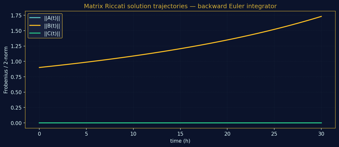
avec conditions terminales $A(T) = 0$, $B(T) = I$, $C(T) = 0$ (mark-to-market à liquidation). Les théorèmes classiques d'existence de solutions de Riccati ne s'appliquent pas — Bergault-Drissi-Guéant utilisent des estimées a priori du contrôle optimal pour obtenir l'existence et l'unicité globales. with terminal conditions $A(T) = 0$, $B(T) = I$, $C(T) = 0$ (mark-to-market liquidation). Classical existence theorems for Riccati equations do not apply — Bergault-Drissi-Guéant use a priori estimates from the optimal control to obtain global existence and uniqueness.

4. Contrôle de feedback optimal $v^\star$Optimal feedback control $v^\star$

Le maximum du Hamiltonien donne immédiatement la vitesse optimale en forme close: Maximising the Hamiltonian immediately yields the closed-form optimal speed:

Trois termes interprétables: Three interpretable terms:

• $\eta^{-1}\,A(t)\,q$ — retour de l'inventaire vers zéro pondéré par le risque cumulatif futur ;inventory pull-back weighted by the cumulative future risk;
• $\eta^{-1}\,\tfrac12(I+B(t))(s-\mu)$ — composante de retour-à-la-moyenne du panier (signal cross-asset) ;basket mean-reversion component (cross-asset signal);
• $\eta^{-1}\,\tfrac12 C(t)$ — terme constant qui s'annule en l'absence de drift de prévision.constant term that vanishes in the absence of a forecast drift.

Figure 1 · Trajectoires des coefficients Riccati $A,B,C$ sur l'horizon de 30 minutes — sortie directe de l'intégrateur RK4 backward du solveur HFThot. Figure 1 · Trajectories of the Riccati coefficients $A,B,C$ over the 30-minute horizon — direct output of HFThot's backward RK4 integrator.

5. Expérience reproductible — LOB Binance liveReproducible experiment — live Binance LOB

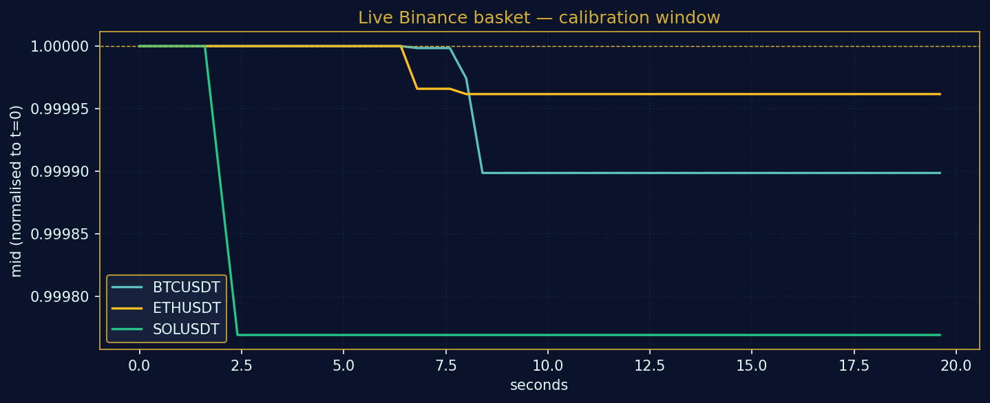
Pour ancrer la théorie dans des données réelles, nous échantillonnons en direct le top-of-book Binance pour le panier {BTCUSDT, ETHUSDT, SOLUSDT}, calibrons la covariance instantanée $\Sigma$ par estimateur réalisé sur 50 mids consécutifs ($\Delta t = 0.4\,s$), et fixons les demi-vies de retour à la moyenne aux échelles littérature (1 h, 30 min, 15 min). Le code complet est versionné dans notebooks/_run_blog_experiment.py. To anchor the theory in real data, we live-sample Binance top-of-book for the basket {BTCUSDT, ETHUSDT, SOLUSDT}, calibrate the instantaneous covariance $\Sigma$ by realised estimator over 50 consecutive mids ($\Delta t = 0.4\,\text{s}$), and pin mean-reversion half-lives to literature-motivated scales (1 h, 30 min, 15 min). Full code is versioned in notebooks/_run_blog_experiment.py.

Figure 2 · Fenêtre de calibration sur 20 secondes — mids normalisés à $t=0$ pour BTCUSDT, ETHUSDT, SOLUSDT. Figure 2 · 20-second calibration window — mids normalised to $t=0$ for BTCUSDT, ETHUSDT, SOLUSDT.

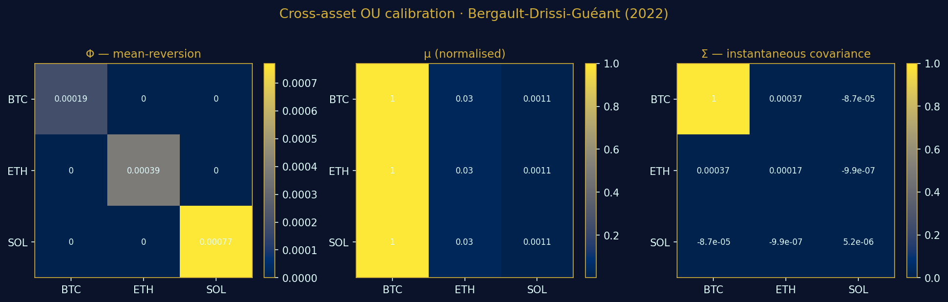
Figure 3 · Heatmaps des paramètres calibrés $\Phi$, $\mu$ (normalisé), $\Sigma$. La diagonale de $\Phi$ encode les demi-vies (1 h / 30 min / 15 min) ; $\Sigma$ révèle les co-mouvements intra-panier. Figure 3 · Heatmaps of the calibrated parameters $\Phi$, $\mu$ (normalised), $\Sigma$. The diagonal of $\Phi$ encodes the half-lives (1 h / 30 min / 15 min); $\Sigma$ reveals intra-basket co-movements.

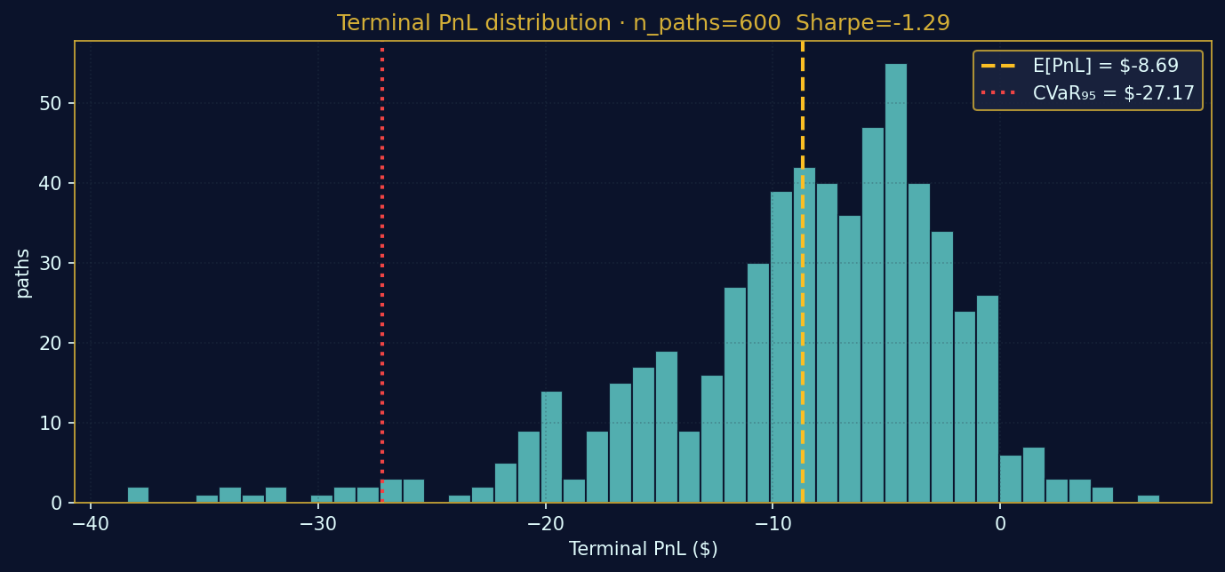
Avec inventaire initial $q_0 = (+0.05\,\text{BTC},\, -0.50\,\text{ETH},\, +5\,\text{SOL})$ — un panier long BTC / short ETH / long SOL typique d'un trader stat-arb intraday — nous simulons 600 trajectoires Monte-Carlo sous le contrôle $v^\star$ avec $\gamma = 10^{-9}$ et $\eta_i = 10^{-4}\,S_i^2$: With initial inventory $q_0 = (+0.05\,\text{BTC},\, -0.50\,\text{ETH},\, +5\,\text{SOL})$ — a typical long BTC / short ETH / long SOL intraday stat-arb basket — we simulate 600 Monte-Carlo paths under the $v^\star$ control with $\gamma = 10^{-9}$ and $\eta_i = 10^{-4}\,S_i^2$:

Figure 4 · Distribution du PnL terminal sur 600 trajectoires Monte-Carlo. Lignes pointillées: $E[\text{PnL}]$ (or) et $\text{CVaR}_{95}$ (rouge). Figure 4 · Terminal PnL distribution across 600 Monte-Carlo paths. Dashed lines: $E[\text{PnL}]$ (gold) and $\text{CVaR}_{95}$ (red).

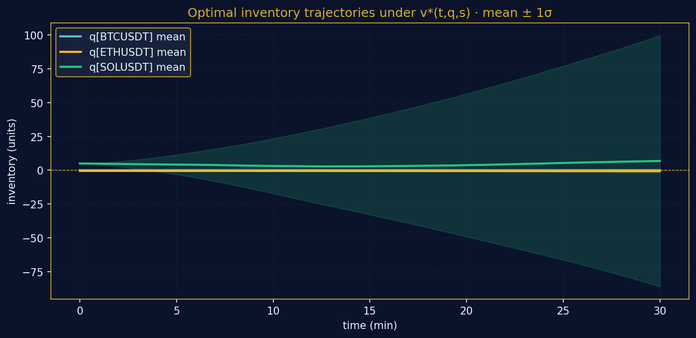
Figure 5 · Trajectoires d'inventaire optimales par actif sous $v^\star(t,q,s)$ — bande $\pm 1\sigma$ Monte-Carlo. La grande dispersion BTC reflète sa volatilité dominante dans $\Sigma$. Figure 5 · Optimal inventory trajectories per asset under $v^\star(t,q,s)$ — Monte-Carlo $\pm 1\sigma$ envelope. The wide BTC dispersion reflects its dominant volatility in $\Sigma$.

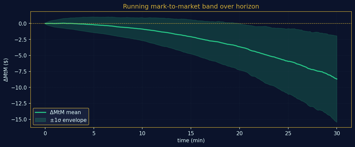
Figure 6 · Bande $\Delta$Mark-to-market sur l'horizon — entonnoir caractéristique d'un programme de liquidation optimal. Figure 6 · $\Delta$Mark-to-market band over the horizon — characteristic funnel of an optimal liquidation programme.

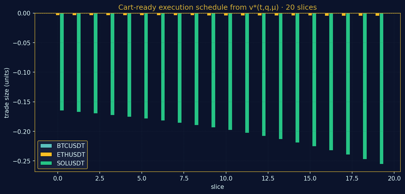
Figure 7 · Planning d'exécution déterministe (20 tranches) issu de $v^\star(t,q,\mu)$ — directement injectable dans le moteur paper-trading HFThot. Figure 7 · Deterministic 20-slice execution schedule from $v^\star(t,q,\mu)$ — directly injectable into the HFThot paper-trading engine.

Une commande Python en trois lignes reproduit toute l'expérience à partir d'un snapshot LOB: A three-line Python snippet reproduces the entire experiment from a LOB snapshot:

from app.services.quant.ou_optimal_execution import (
    OUParams, solve_riccati, simulate, build_execution_schedule,
)

params  = OUParams(Phi=Phi_diag, mu=s_mean, Sigma=Sigma_realised, dt_seconds=0.4)
sol     = solve_riccati(params=params, eta=eta_mat, horizon_seconds=1800,
                        n_steps=240, gamma=1e-9)
result  = simulate(sol=sol, q0=q0, s0=s_now, n_paths=600, rng_seed=42)
schedule = build_execution_schedule(sol, q0=q0, s_now=s_now, n_slices=20)
print(result.expected_pnl, result.std_pnl, result.sharpe, result.cvar95)

6. Calibration multi-fréquence & estimateur de Hayashi-YoshidaMulti-frequency calibration & the Hayashi-Yoshida estimator

Échantillonner à pas fixe $\Delta t$ d'un panier hétérogène est biaisé: BTC tique 5–10× plus vite que SOL, et l'effet Epps fait s'effondrer la corrélation observée à mesure que $\Delta t \to 0$. Pour une covariance instantanée non-biaisée sur un panier multi-actifs, nous utilisons l'estimateur de Hayashi-Yoshida (2005) — somme des produits de retours sur tous les intervalles temporels qui se chevauchent, sans aucune synchronisation préalable: Sampling a heterogeneous basket at fixed $\Delta t$ is biased: BTC ticks 5–10× faster than SOL, and the Epps effect collapses observed correlation as $\Delta t \to 0$. For an unbiased instantaneous covariance on a multi-asset basket, we use the Hayashi-Yoshida (2005) estimator — sum of return products over all overlapping time intervals, with no prior synchronisation:

où $\Delta r_i^{(k)}$ est le log-retour de l'actif $i$ sur son $k$-ième intervalle natif $I_i^{(k)}$. L'estimateur est convergent sous échantillonnage non-synchrone et asymptotiquement gaussien — propriétés cruciales pour un panier crypto où chaque venue émet des updates à des cadences différentes. where $\Delta r_i^{(k)}$ is the log-return of asset $i$ over its $k$-th native interval $I_i^{(k)}$. The estimator is consistent under non-synchronous sampling and asymptotically Gaussian — critical properties for a crypto basket where each venue emits updates at different cadences.

Pondération multi-fréquence de ΦMulti-frequency weighting of Φ

Plutôt qu'une demi-vie unique, nous décomposons la matrice de retour à la moyenne en composantes spectrales avec poids $w_h$ par bande de fréquence: Rather than a single half-life, we decompose the mean-reversion matrix into spectral components with weights $w_h$ per frequency band:

avec $\mathcal{H} = \{\text{1 min},\, \text{5 min},\, \text{30 min},\, \text{1 h}\}$ couvrant le spectre micro→méso. Les poids sont estimés par moindres carrés sur le spectre empirique de la covariance des retours. with $\mathcal{H} = \{\text{1 min},\, \text{5 min},\, \text{30 min},\, \text{1 h}\}$ covering the micro→meso spectrum. Weights are estimated by least squares on the empirical return-covariance spectrum.

7. Options court-terme: accélérateur d'espérance de PnLShort-term options: an E[PnL] accelerator

Le contrôle $v^\star$ minimise le coût d'impact sur l'espace des quantités linéaires. Mais l'espérance de PnL d'un programme d'exécution multi-actif peut être strictement augmentée en superposant un overlay d'options court-terme (DTE 0–7) qui exploite la convexité du payoff face à la dynamique OU. The $v^\star$ control minimises impact cost on the linear-quantity space. But the expected PnL of a multi-asset execution programme can be strictly increased by overlaying short-dated options (0–7 DTE) that exploit payoff convexity against OU dynamics.

Décomposition de l'espérance de PnLE[PnL] decomposition

Soit $\Pi_t = X_t + q_t \cdot S_t + \Theta_t$ la valeur totale, avec $\Theta_t$ la valeur de marché de l'overlay d'options. L'espérance de la variation infinitésimale s'écrit (lemme d'Itô + valorisation Black-Scholes locale): Let $\Pi_t = X_t + q_t \cdot S_t + \Theta_t$ be the total value, with $\Theta_t$ the mark-to-market of the option overlay. The expected infinitesimal change reads (Itô's lemma + local Black-Scholes pricing):

où $\Gamma_t = \partial^2 \Theta_t / \partial S^2$ est la matrice gamma (Hessien de la valeur d'options par rapport au prix sous-jacent) et $\Theta^{\Theta}_t = \partial \Theta_t / \partial t$ le theta agrégé. La moisson gamma $\tfrac12\,\mathrm{tr}(\Gamma\Sigma)$ est strictement positive pour des positions long-gamma et croît avec la volatilité réalisée — précisément ce que la dynamique OU produit lors des phases de retour à la moyenne. where $\Gamma_t = \partial^2 \Theta_t / \partial S^2$ is the gamma matrix (Hessian of option value w.r.t. underlying) and $\Theta^{\Theta}_t = \partial \Theta_t / \partial t$ the aggregate theta. The gamma harvest $\tfrac12\,\mathrm{tr}(\Gamma\Sigma)$ is strictly positive for long-gamma positions and grows with realised volatility — precisely what OU dynamics produce during mean-reversion phases.

Programme d'optimisation augmentéAugmented optimisation programme

$\theta$ représente le vecteur de poids d'options (deltas et gammas par tenor), et la contrainte de break-even gamma-vs-theta garantit que la moisson gamma surpasse la décroissance temporelle d'au moins $\kappa$. Sous l'ansatz quadratique étendu pour $J$, le contrôle optimal couplé devient: $\theta$ is the option weight vector (deltas and gammas per tenor), and the gamma-vs-theta break-even constraint ensures gamma harvest exceeds time decay by at least $\kappa$. Under the extended quadratic ansatz for $J$, the coupled optimal control becomes:

Le terme additionnel $\Sigma\Gamma_t\mathbf{1}$ réoriente l'exécution vers les actifs où la convexité du payoff combinée à la covariance instantanée maximise localement le drift de PnL. The additional term $\Sigma\Gamma_t\mathbf{1}$ reorients execution toward assets where payoff convexity combined with instantaneous covariance locally maximises the PnL drift.

8. Extension adaptative cross-pool (Baldacci-Manziuk 2020)Adaptive extension across liquidity pools (Baldacci-Manziuk 2020)

Bergault-Drissi-Guéant suppose une dynamique OU statique. En réalité, l'imbalance et le spread d'un même actif varient entre venues (Binance vs Coinbase vs OKX), et la distribution conditionnelle des fills dépend de la profondeur instantanée de chaque pool. Bergault-Drissi-Guéant assumes static OU dynamics. In practice, imbalance and spread of the same asset vary across venues (Binance vs Coinbase vs OKX), and the conditional fill distribution depends on the instantaneous depth of each pool.

Baldacci & Manziuk (2020) proposent un cadre Bayésien adaptatif où les paramètres du modèle (drift, intensité d'arrivée, profondeur) sont mis à jour en temps réel à partir des observations. Le contrôle stochastique est résolu par différences finies ou par deep RL selon la complexité ; les extensions naturelles incluent les signaux short/long, l'impact de marché et la liquidité cachée. Baldacci & Manziuk (2020) propose an adaptive Bayesian framework where model parameters (drift, arrival intensity, depth) are updated in real time from observations. The stochastic control problem is solved by finite differences or by deep reinforcement learning depending on complexity; natural extensions include short/long signals, market impact and hidden liquidity.

9. Industrialisation dans HFThot ThotCloud LabIndustrialisation in HFThot ThotCloud Lab

Le solveur OU multi-actif est intégré dans la page Streamlit 🔬 Microstructure Lab (onglet 🎯 OU optimal execution) et sert le pipeline complet: The multi-asset OU solver is integrated in the Streamlit page 🔬 Microstructure Lab (tab 🎯 OU optimal execution) and powers the complete pipeline:

1. Multi-select de panier avec parsing CCXT natif (BTC/ETH/SOL/AVAX/...).Basket multi-select with native CCXT parsing (BTC/ETH/SOL/AVAX/...).
2. Échantillonneur historique persistant en session_state.Calibration history sampler persisted in session_state.
3. Demi-vies par actif affichées et éditables.Per-asset half-lives displayed and editable.
4. Dropdowns Objectif (Mean-variance / Min-variance / Max-PnL) et Horizon (5 min / 30 min / EOD / EOW / Custom).Objective dropdown (Mean-variance / Min-variance / Max-PnL) and Horizon dropdown (5 min / 30 min / EOD / EOW / Custom).
5. Inputs $\gamma$ et $\eta$ pour ajuster aversion au risque et impact.$\gamma$ and $\eta$ inputs for risk aversion and impact tuning.
6. Vecteur d'inventaire $q_0$ et nombre de trajectoires.Inventory vector $q_0$ and number of paths.
7. Bouton Solve+Simulate → dashboard 4-KPI + 3 graphes Plotly + bouton 🛒 Add to cart vers paper-trading.Solve+Simulate button → 4-KPI dashboard + 3 Plotly charts + 🛒 Add-to-cart button to paper-trading.

Plans HFThot et accès aux fonctionnalitésHFThot tiers & feature access

10. Aller plus loin: cours prérequis & notebook approfondiGo deeper: prerequisites course & advanced notebook

Cet article suppose une familiarité avec le contrôle stochastique et le calcul d'Itô multidimensionnel. Pour les lecteurs souhaitant tout reconstruire à partir de zéro — du lemme d'Itô à la dérivation complète des EDOs Riccati matricielles, en passant par Hayashi-Yoshida et la valorisation rough-Heston — nous publions deux ressources commerciales complémentaires: This article assumes familiarity with stochastic control and multi-dimensional Itô calculus. For readers wishing to rebuild everything from scratch — from Itô's lemma to the full derivation of matrix Riccati ODEs, including Hayashi-Yoshida and rough-Heston pricing — we publish two complementary commercial resources:

11. RéférencesReferences

1. Bergault, P., Drissi, F. & Guéant, O. (2022). Multi-asset optimal execution and statistical arbitrage strategies under Ornstein-Uhlenbeck dynamics. SIAM Journal on Financial Mathematics, 13(1), 353–390.
2. Baldacci, B. & Manziuk, I. (2020). Adaptive trading strategies across liquidity pools. arXiv:2008.07807 [q-fin.TR].
3. Almgren, R. & Chriss, N. (2001). Optimal execution of portfolio transactions. Journal of Risk, 3(2), 5–40.
4. Avellaneda, M. & Stoikov, S. (2008). High-frequency trading in a limit order book. Quantitative Finance, 8(3), 217–224.
5. Hayashi, T. & Yoshida, N. (2005). On covariance estimation of non-synchronously observed diffusion processes. Bernoulli, 11(2), 359–379.
6. Cartea, Á., Jaimungal, S. & Penalva, J. (2015). Algorithmic and High-Frequency Trading. Cambridge University Press.