📖 Abstract
Yang–Mills theory describes three of the four fundamental forces. It works: its predictions are confirmed to ten significant figures. And yet nobody has proved it mathematically exists. The Yang–Mills mass gap is one of the Clay Institute's seven Millennium Prize Problems — one million dollars, still unclaimed.
This article starts from zero: what a gauge symmetry is, why moving from an abelian to a non-abelian group changes everything, and why that non-commutativity is precisely the source of the difficulty. We then connect the problem to the Higgs boson and to high-frequency gravitational waves. Computable quantities are evaluated with pysic-rs.
📋 Table of Contents
- Preliminaries: what is a gauge?
- From Maxwell to Yang–Mills: non-commutativity
- The action and the field equations
- History: 1954–2000
- The mass gap: the exact statement
- Asymptotic freedom and instantons
- Topological charge and θ-vacua
- The Higgs connection
- The high-frequency gravitational-wave connection
- pysic-rs code recipes
- Recap
- References
1. Preliminaries: what is a gauge?
Start with the simplest case, assuming nothing. In quantum mechanics an electron's state is a complex wavefunction $\psi(x)$. Every observable depends on $|\psi|^2$. Multiplying $\psi$ by a constant phase $e^{i\alpha}$ therefore changes nothing measurable.
Here is Weyl's question, later taken up by Yang and Mills: what if the phase could vary from point to point? Demand that
$$\psi(x) \;\longmapsto\; e^{i\alpha(x)}\,\psi(x)$$leaves the physics invariant. The problem shows up immediately in the derivative: $\partial_\mu\psi$ no longer transforms cleanly, because the Leibniz rule produces a spurious term $i(\partial_\mu\alpha)\psi$. The only way to repair this is to introduce a compensating field $A_\mu$ and replace the ordinary derivative by the covariant derivative:
$$D_\mu = \partial_\mu + i g A_\mu, \qquad A_\mu \longmapsto A_\mu - \tfrac{1}{g}\partial_\mu\alpha$$Key takeaway: the electromagnetic field is not postulated, it is forced. Demanding local phase invariance requires the photon to exist. That is the gauge principle, and it is the most beautiful idea in twentieth-century physics.
The phases $e^{i\alpha}$ form the group $U(1)$: a circle. Two phases always commute, $e^{i\alpha}e^{i\beta}=e^{i\beta}e^{i\alpha}$. We say $U(1)$ is abelian. All of electrodynamics follows from that circle.
2. From Maxwell to Yang–Mills: non-commutativity
In 1954, Chen Ning Yang and Robert Mills asked a disarmingly simple question: what if the group were not a circle but something bigger — $SU(2)$, $SU(3)$ — whose elements do not commute?
The gauge field then becomes matrix-valued: $A_\mu = A_\mu^a T^a$, where the $T^a$ are the Lie-algebra generators. Their non-commutativity is encoded by the structure constants $f^{abc}$:
$$[T^a, T^b] = i f^{abc} T^c$$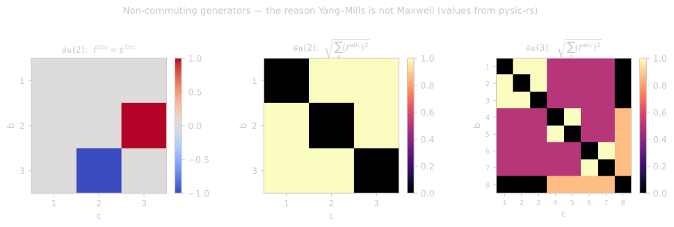
The consequence is spectacular. The field-strength tensor acquires an extra term, quadratic in the field itself:
$$F_{\mu\nu} = \partial_\mu A_\nu - \partial_\nu A_\mu + i g\,[A_\mu, A_\nu]$$The heart of the problem. This commutator $[A_\mu,A_\nu]$ is absent in electrodynamics (it vanishes for an abelian group). Its presence means the gauge field interacts with itself. Photons ignore one another; gluons bind to each other. The equation becomes non-linear, and the entire mathematical difficulty follows from that.
3. The action and the field equations
The Yang–Mills action is the simplest gauge-invariant, Lorentz-invariant quantity one can build from $F_{\mu\nu}$:
$$S_{\rm YM} = -\frac{1}{4}\int d^4x\; F^a_{\mu\nu}F^{a\,\mu\nu}$$One point that is often lost in numerical implementations: this action is quadratic in $F$. Replacing $F \to \lambda F$ gives $S \to \lambda^2 S$. That is an elementary but ruthlessly effective check on a solver — we use exactly this as a regression test in pysic-rs.
Varying the action gives the field equations. They resemble Maxwell's equations with one decisive difference: the derivative is covariant, so the equation is non-linear.
$$D_\mu F^{\mu\nu} = \partial_\mu F^{\mu\nu} + ig[A_\mu, F^{\mu\nu}] = J^\nu$$Reminder — side by side:
| Maxwell — $U(1)$ | Yang–Mills — $SU(N)$ | |
|---|---|---|
| Group | abelian | non-abelian |
| $F_{\mu\nu}$ | $\partial_\mu A_\nu-\partial_\nu A_\mu$ | $+\;ig[A_\mu,A_\nu]$ |
| Self-interaction | no | yes |
| Coupling at high energy | grows | shrinks |
| Lightest quantum | photon, massless | glueball, massive (?) |
4. History: 1954–2000
1954. Yang presents the theory at Princeton. Wolfgang Pauli interrupts: “What is the mass of this field?” Yang has no answer. The theory predicts massless gauge bosons, like the photon — yet no infinite-range force is observed beyond electromagnetism and gravity. Pauli presses so hard that Yang sits down. The paper is published anyway and remains, for a decade, a mathematical curiosity.
1964. Higgs, Englert and Brout show that a scalar field can give mass to gauge bosons without breaking gauge invariance. Pauli's objection finally has an answer.
1971–72. 't Hooft and Veltman prove that broken non-abelian gauge theories are renormalisable. The theory becomes computable.
1973. Gross, Wilczek and Politzer discover asymptotic freedom: in Yang–Mills the coupling decreases at high energy. This is the opposite of electrodynamics, and it explains why quarks look free in violent collisions while remaining confined at rest. Nobel Prize 2004.
2000. The Clay Institute lists the Yang–Mills mass gap among its seven Millennium Problems. The official statement is written by Arthur Jaffe and Edward Witten. It remains open.
5. The mass gap: the exact statement
The problem asks for two things, and it is essential to keep them apart.
(i) Existence. Construct a quantum Yang–Mills field theory on $\mathbb{R}^4$ for a compact simple gauge group, satisfying the Wightman (or Osterwalder–Schrader) axioms. In other words: show that the object whose predictions physicists have been computing for fifty years exists as a well-defined mathematical object.
(ii) The gap. Prove there exists a constant $\Delta > 0$ such that every non-vacuum state has energy at least $\Delta$. The Hamiltonian's spectrum must have a hole above the vacuum:
$$\operatorname{spec}(H) \subseteq \{0\} \cup [\Delta, \infty), \qquad \Delta > 0$$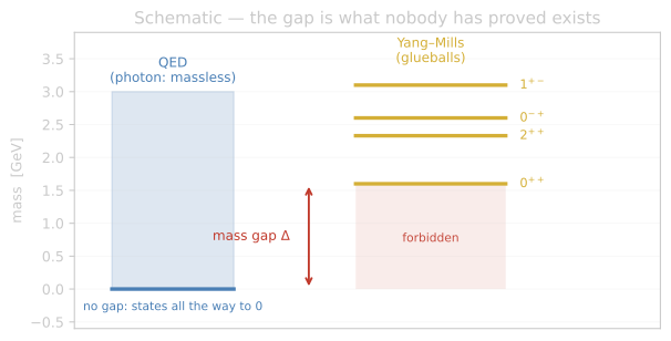
Why it is hard. Lattice simulations measure $\Delta \approx 1.6$ GeV to a few percent. But a lattice is finite and discrete; the problem demands the continuum limit on $\mathbb{R}^4$, where all control is lost. In two and three dimensions the construction has been carried out. In four — ours — the coupling is dimensionless, the theory sits exactly at the edge of renormalisability, and no known method controls the limit. Confinement and the gap are non-perturbative: Feynman series, which give ten exact digits at high energy, say nothing whatsoever here.
6. Asymptotic freedom and instantons
The Yang–Mills coupling depends on the energy scale. To one loop:
$$\alpha_s(Q) = \frac{1}{b_0\,\ln(Q^2/\Lambda^2)}, \qquad b_0 = \frac{33 - 2 n_f}{12\pi}$$The sign of $b_0$ changes everything. For $n_f < 16.5$ quark flavours, $b_0 > 0$ and the coupling decreases as $Q$ grows. That is asymptotic freedom. Conversely, at low energy the coupling blows up towards $\Lambda \approx 200$ MeV — precisely where perturbation theory dies and confinement begins.
Instantons are classical solutions of the Euclidean equation, self-dual ($F = \tilde F$), which tunnel the vacuum from one topological sector to another. Their action is remarkably simple:
$$S_{\rm inst} = \frac{8\pi^2}{g^2}, \qquad \text{amplitude} \sim e^{-S_{\rm inst}} = e^{-8\pi^2/g^2}$$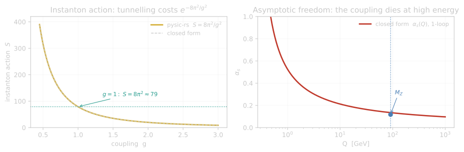
instanton_action), overlaid on the closed form. At $g=1$, $S\approx79$: the amplitude $e^{-79}$ is astronomically small, which is why instanton effects are invisible in perturbation theory. Right: the one-loop running coupling (closed form), with the measured $\alpha_s(M_Z)\approx0.118$.
7. Topological charge and θ-vacua
The Yang–Mills vacuum is not unique. Gauge configurations fall into sectors labelled by an integer — the topological charge, or winding number:
$$Q = \frac{g^2}{32\pi^2}\int d^4x\; \epsilon^{\mu\nu\rho\sigma}F^a_{\mu\nu}F^a_{\rho\sigma} \;\in\; \mathbb{Z}$$This quantisation is not a computational accident: it comes from topology. A winding cannot change continuously. It is exactly the same mechanism as the winding number of a plane curve, or a skyrmion's charge — objects pysic-rs computes directly and which we validate against their exact values.
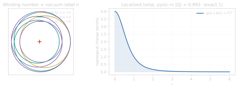
winding_number) — the integer labelling a vacuum sector. Right: topological charge density of a localised lump, $q(r)=4/(1+r^2)^2$, whose total charge comes out as $|Q|=0.993$ against the exact value 1 (skyrmion_number).
Since all sectors are physically reachable by tunnelling, the true vacuum is a superposition weighted by an angle $\theta$: $|\theta\rangle = \sum_n e^{in\theta}|n\rangle$. That angle permits a CP-violating term in the Lagrangian. Experiment, however, requires $|\theta| < 10^{-10}$. Why so small? This is the strong CP problem, a second open mystery born of the same topological structure.
8. The Higgs connection
A very common confusion needs clearing up here. The Higgs mechanism and the Yang–Mills mass gap both produce mass, but they are distinct phenomena.
The Higgs works by spontaneous symmetry breaking. A scalar field acquires a vacuum expectation value, $\langle\phi\rangle = v \approx 246$ GeV, and the gauge bosons “eat” the Goldstone degrees of freedom to become massive: $m_W = \tfrac12 g v$. This is perturbative, computable, and it is what the LHC confirmed in 2012.
The Yang–Mills gap needs no scalar field at all. In pure QCD, with no Higgs whatsoever, the theory generates its own mass scale — dimensional transmutation. The classical Lagrangian contains no mass and is scale-invariant; the quantum theory nonetheless produces $\Lambda \approx 200$ MeV and a glueball at 1.6 GeV. It is this purely non-perturbative phenomenon that nobody knows how to prove.
In one sentence: the Higgs explains the mass of the $W$ and $Z$; the Yang–Mills gap would explain why the proton weighs 938 MeV when its quarks account for barely ten. Most of your mass does not come from the Higgs, but from the binding energy of a non-abelian gauge field — that is, from precisely the phenomenon nobody has proved.
9. The high-frequency gravitational-wave connection
LIGO and Virgo observe gravitational waves between 10 Hz and a few kHz — compact-object mergers. High-frequency gravitational waves (HFGW), above the MHz, are a different animal: no known astrophysical object radiates there. Any detection would be a signature of fundamental physics, and several candidate sources are directly Yang–Mills in nature.
The reason is a matter of scale. A phase transition in the early universe at temperature $T$ produces a gravitational-wave background whose frequency today is, in order of magnitude,
$$f_0 \;\sim\; 10^{-8}\,\mathrm{Hz} \times \left(\frac{T}{1\ \mathrm{GeV}}\right)$$The QCD deconfinement transition, near $T \approx 150$ MeV, therefore lands in the nanohertz band — the one pulsar-timing arrays probe. A gauge transition at a much higher scale, however (a confining dark sector, grand-unification breaking), projects into the MHz–GHz range: the HFGW band.
Three mechanisms therefore tie Yang–Mills to HFGW. First, a first-order phase transition in a gauge sector produces colliding bubbles, a violent source of gravitational waves. Second, topological defects — strings, walls, monopoles — are exactly the objects classified by the topological charges of §7; their collapse radiates at high frequency. Third, the signal amplitude depends on the order of the transition, which depends on the theory's spectrum — hence on the gap. Deciding whether a gauge sector yields a detectable HFGW background is, in part, a question about its mass gap.
Required honesty: no HFGW has been detected to date. Resonant cavities and electromagnetic-conversion detectors are at prototype stage, and current sensitivities sit well above the predictions. The connection described here is theoretically sound but experimentally prospective.
10. pysic-rs code recipes
Honest scope. The recipes below call only routines covered by passing closed-form tests. The Yang–Mills core of pysic-rs (field strength, connections, Wilson loops) is under repair: our own invariant tests revealed that the implemented action was linear in $F$ instead of quadratic, and that $F_{\mu\nu}$ was not antisymmetric. We do not publish results produced by unvalidated code.
Non-commutativity, explicitly
import numpy as np
from pysicrs import su2_structure_constants, su3_structure_constants

f2 = np.array(su2_structure_constants())   # 3x3x3
f3 = np.array(su3_structure_constants())   # 8x8x8

print("su(2) non-zero:", int((abs(f2) > 1e-12).sum()))   # 6  = 1 triple x 3!
print("su(3) non-zero:", int((abs(f3) > 1e-12).sum()))    # 54 = 9 triples x 3!

# Total antisymmetry is the defining property: f^abc = -f^bac
print("antisymmetric:", np.allclose(f3, -f3.transpose(1, 0, 2)))   # True

# Jacobi identity - the statement that the algebra closes
J = np.einsum('ade,bcd->abce', f3, f3) \
  + np.einsum('bde,cad->abce', f3, f3) \
  + np.einsum('cde,abd->abce', f3, f3)
print("Jacobi residual:", abs(J).max()) # ~1e-16The cost of an instanton
import math
from pysicrs import instanton_action

for g in (0.5, 1.0, 2.0):
    S = instanton_action(g)
    print(f"g={g}:  S={S:8.3f}   e^-S={math.exp(-S):.3e}")

# g=0.5:  S= 315.827   e^-S=0.000e+00   <- tunnelling utterly suppressed
# g=1.0:  S=  78.957   e^-S=5.20e-35
# g=2.0: S= 19.739 e^-S=2.67e-09 <- strong coupling: instantons matterThe topological charge of a vacuum
import math
from pysicrs import winding_number, skyrmion_number

# A loop in the gauge group, traversed n times -> vacuum label n
for n in (1, 2, -3):
    ts = [2*math.pi*i/2000 for i in range(2000)]
    f1 = [math.cos(n*t) for t in ts]
    f2 = [math.sin(n*t) for t in ts]
    print(f"n={n:+d} -> winding {winding_number(f1, f2):+.0f}")

# A localised self-dual lump carries exactly one unit of charge
span, npts = 16.0, 641
xs = [-span + 2*span*i/(npts-1) for i in range(npts)]
h = xs[1] - xs[0]
field = [[[2*x/(x*x+y*y+1), 2*y/(x*x+y*y+1), (x*x+y*y-1)/(x*x+y*y+1)]
          for y in xs] for x in xs]
print(f"|Q| = {abs(skyrmion_number(field, h, h)):.4f}")   # 0.9951 (exact: 1)
11. Recap
- Demanding local phase invariance forces a gauge field to exist. Electromagnetism is not postulated, it is deduced.
- Replacing $U(1)$ by a non-abelian group adds $ig[A_\mu,A_\nu]$ to $F_{\mu\nu}$: the field self-interacts and the equation turns non-linear.
- The action $S=-\tfrac14\int F^a_{\mu\nu}F^{a\mu\nu}$ is quadratic in $F$ — an elementary and merciless regression test.
- The Millennium Problem asks two things: axiomatic existence on $\mathbb{R}^4$ and a gap $\Delta>0$ in the spectrum.
- The lattice measures $\Delta\approx1.6$ GeV; nobody can control the continuum limit in four dimensions.
- Higgs $\neq$ mass gap. The Higgs gives the $W$ its mass; the gap would explain the proton's — hence yours.
- The integer topological charges labelling the vacua are computable today, and they connect Yang–Mills to high-frequency gravitational-wave backgrounds.
This article assumes little, but it moves fast. For readers who want to rebuild gauge theory from the foundations — from Lie groups to principal bundles, from the covariant derivative to the Yang–Mills action, with every computation carried through — we publish an introductory course.
Introductory course — Gauge Theory & Yang–Mills
10,99 €One-off purchase, lifetime access · 30 pages. LaTeX course with TikZ and pgfplots, no gaps in the progression: Lie groups and algebras → $U(1)$ and the covariant derivative → non-abelian groups and structure constants → field strength and the Bianchi identity → the Yang–Mills action and field equations → instantons and topological sectors. Companion notebook using pysic-rs.
Table of contents (6 chapters + 3 appendices)
- Lie groups and algebras: the useful minimum
- $U(1)$, local phase, covariant derivative
- $SU(2)$, $SU(3)$ and the structure constants
- Field strength, Bianchi identity, duality
- Yang–Mills action, variation, field equations
- Instantons, winding number, $\theta$-vacua
12. References
- C. N. Yang & R. L. Mills, Conservation of Isotopic Spin and Isotopic Gauge Invariance, Phys. Rev. 96, 191 (1954).
- A. Jaffe & E. Witten, Quantum Yang–Mills Theory, Clay Mathematics Institute Millennium Prize Problem official description (2000).
- D. J. Gross & F. Wilczek, Ultraviolet Behavior of Non-Abelian Gauge Theories, Phys. Rev. Lett. 30, 1343 (1973).
- H. D. Politzer, Reliable Perturbative Results for Strong Interactions?, Phys. Rev. Lett. 30, 1346 (1973).
- P. W. Higgs, Broken Symmetries and the Masses of Gauge Bosons, Phys. Rev. Lett. 13, 508 (1964).
- F. Englert & R. Brout, Broken Symmetry and the Mass of Gauge Vector Mesons, Phys. Rev. Lett. 13, 321 (1964).
- G. 't Hooft & M. Veltman, Regularization and Renormalization of Gauge Fields, Nucl. Phys. B 44, 189 (1972).
- A. A. Belavin, A. M. Polyakov, A. S. Schwartz & Yu. S. Tyupkin, Pseudoparticle Solutions of the Yang–Mills Equations, Phys. Lett. B 59, 85 (1975).
- K. G. Wilson, Confinement of Quarks, Phys. Rev. D 10, 2445 (1974).
- C. J. Morningstar & M. Peardon, The Glueball Spectrum from an Anisotropic Lattice Study, Phys. Rev. D 60, 034509 (1999).
- N. Aggarwal et al., Challenges and Opportunities of Gravitational-Wave Searches at MHz to GHz Frequencies, Living Rev. Relativ. 24, 4 (2021).
- C. Caprini & D. G. Figueroa, Cosmological Backgrounds of Gravitational Waves, Class. Quantum Grav. 35, 163001 (2018).
- M. E. Peskin & D. V. Schroeder, An Introduction to Quantum Field Theory, Addison-Wesley (1995), chapters 15–17.
- pysic-rs documentation — gauge theory, topology.
Want to go deeper?
This article moves fast, by design. A 29-page companion primer builds, from first principles, all the machinery assumed here: Lie groups and algebras, principal bundles, connections and curvature, the variational derivation of the Yang–Mills field equations, the Wightman axioms needed to state the Clay Millennium Problem rigorously, asymptotic freedom, instantons, and the Higgs mechanism — with full derivations, worked examples, and exercises with solutions.
Read the prerequisites (PDF) All our papers